Supervised Learning Glossary - 50+ terms you should know

Dive into the world of Supervised Learning with our comprehensive glossary of over 50 essential terms you need to know! Whether you’re a seasoned expert or just starting your journey into the fascinating realm of Artificial Intelligence and Machine Learning, this glossary will serve as a valuable resource to enhance your understanding and deepen your knowledge of Supervised Learning.

We’ve meticulously organized the terms into related categories, providing you with a clearer and more holistic view of the Supervised Learning landscape. To help you navigate through the plethora of concepts, we’ve included cross-references and links between terms, enabling you to seamlessly move from one idea to another.

Don’t forget to explore our other glossaries, diving into the intricate subfields of AI and ML:

Now, let’s embark on this exciting journey and unravel the intricate world of Supervised Learning!

1. Supervised Learning

Supervised learning is a type of machine learning in which a model learns patterns and relationships from a dataset containing both input features and corresponding output labels. In supervised learning, the objective is to train the model to predict the correct output labels for new, unseen data based on the input features. This learning paradigm is called “supervised” because the model is guided by the correct answers, or labels, during the training process.

Common supervised learning tasks include regression, where the model predicts continuous numeric values, and classification, where the model assigns input data to discrete categories. To train a supervised learning model, the algorithm iteratively adjusts its parameters to minimize the difference between its predictions and the actual labels in the dataset. This process typically involves using loss functions and optimization algorithms to measure the error and update the model’s parameters, respectively. Once trained, the model can make predictions on new data by processing their features through the learned relationships between input features and output labels.

2. Dataset

A dataset is a collection of data points used in machine learning and statistics. These data points are usually represented as a table, where each row corresponds to an individual observation, sample, or data point, and each column represents a feature or variable associated with that observation. In supervised learning, the data points are also associated with labels. Datasets are used to train, validate, and evaluate machine learning models.

3. Training Data

Training data is a subset of the dataset used to train a machine learning model. The model learns from this data by adjusting its parameters to minimize the error between the predicted outputs and the actual outputs.

For example, given a dataset of housing prices with features such as square footage, location, and number of bedrooms, the training data might include 70% of the dataset to allow the model to learn the relationship between these features and the housing prices.

4. Validation Data

Validation data is another subset of the dataset, separate from the training data, used to tune hyperparameters and validate the performance of a machine learning model during the training process. The validation data helps prevent overfitting by providing a way to measure the model’s performance on unseen data while adjusting hyperparameters.

For example, using 15% of the housing prices dataset as validation data helps assess how well the model generalizes to new data and aids in selecting the best hyperparameters.

5. Test Data

Test data is a third, separate, subset of the dataset reserved for evaluating the final performance of a machine learning model after it has been trained and hyperparameters have been tuned. The test data should not be used during training or hyperparameter tuning to ensure an unbiased assessment of the model’s ability to generalize to new, unseen data.

In the housing prices example, the remaining 15% of the dataset could be used as test data to evaluate the model’s performance.

6. Cross-Validation

Cross-validation is a technique used to assess the performance and generalization ability of a machine learning model. In cross-validation, the dataset is divided into a fixed number of equally sized “folds”. The model is then trained and validated multiple times, each time using a different fold as the validation data and the remaining folds as the training data. The model’s performance is averaged across all iterations to provide a more reliable estimate of its generalization ability. Cross-validation helps to reduce the impact of sampling bias and provides a more accurate assessment of the model’s performance.

In summary, the dataset is split into training, validation, and test data to train, tune hyperparameters, and evaluate machine learning models, respectively. Cross-validation is a technique used to provide a more reliable assessment of a model’s performance by using different subsets of the data for training and validation in multiple iterations. These concepts are all related as they are essential components of the model development process, aimed at building models that can generalize well to new, unseen data.

7. Features and 8. Labels

Features and labels are two essential components of a dataset used in supervised machine learning.

Features, also known as independent variables or predictors, are the input data points or attributes used to make predictions or determine the outcome of a machine learning model. They are the characteristics or properties of the data that the model uses to learn patterns and relationships. Features can be numerical (e.g., age, height, temperature) or categorical (e.g., color, gender, product type). In a tabular dataset, features are typically represented as columns.

For example, in a dataset of real estate prices, features could include the number of bedrooms, square footage, location, and age of the property.

Labels, also known as dependent variables, target variables, or ground truth, are the output values or outcomes that a machine learning model aims to predict or classify. In supervised learning, labels are provided in the training dataset, allowing the model to learn the relationship between the features and the labels. Labels can be either continuous (e.g., housing prices) or discrete (e.g., spam or not-spam).

Continuing with the real estate prices example, the label would be the actual price of the property.

In supervised learning, the goal is to create a model that can accurately predict labels based on the features. By training the model with a dataset containing both features and labels, the model learns the underlying patterns and relationships between them, which can then be used to make predictions on new, unseen data.

9. Loss Function

A loss function, also known as a cost function or objective function, is a mathematical function that quantifies the difference between the output predicted by a machine learning model and the correct output (ground truth). It is a critical component of the learning process, as it measures the performance of the model and serves as the basis for optimization during training.

The goal of a machine learning algorithm is to minimize the loss function by adjusting the model’s parameters (e.g., weights and biases in a neural network) iteratively. The choice of loss function depends on the type of problem being solved and the algorithm being used. Some common loss functions include:

Mean Squared Error (MSE): Commonly used for regression problems, it calculates the average of the squared differences between the predicted and actual values. MSE is sensitive to outliers, as it penalizes large errors more heavily than small errors.
Mean Absolute Error (MAE): Also used for regression problems, it calculates the average of the absolute differences between the predicted and actual values. MAE is less sensitive to outliers compared to MSE.
Cross-Entropy Loss: Widely used for classification problems, it measures the difference between the predicted probability distribution and the true probability distribution for the target classes. A smaller cross-entropy loss indicates better performance.
Hinge Loss: Commonly used for Support Vector Machines (SVMs) and some other classification problems, it measures the error between the predicted class and the true class by considering the margin between them. Hinge loss encourages a large margin between different classes, improving classification performance.

The choice of an appropriate loss function is crucial for the success of a machine learning model, as it directly influences the learning process and the quality of the final predictions. The loss function should be tailored to the specific problem and the characteristics of the data being used.

10. Classification

Classification is a type of supervised learning task where the goal is to assign input data to one of several discrete categories or classes. The input data, often represented as feature vectors, is used to train a classification model, which learns the relationship between the features and their corresponding class labels. The objective is to develop a model that can accurately categorize new, unseen data based on the patterns and relationships it has learned during the training process.

For example, consider a dataset of handwritten digits, where each digit is represented by a set of pixel values (features) and has an associated class label indicating the digit’s numerical value (0-9). A classification model, such as a support vector machine or a convolutional neural network, can be trained on this dataset to recognize and classify unseen handwritten digits. The model learns the underlying patterns and characteristics of the digit images during the training process, enabling it to predict the correct class labels for new, unseen handwritten digit images. In this scenario, the classification task involves assigning each input image to one of the ten possible classes (0-9) based on its features.

11. Binary Classification and 12. Multi-Class Classification

Binary classification is a fundamental task in machine learning and pattern recognition, where the goal is to categorize an input into one of two possible classes. In this type of classification, the model predicts whether an input belongs to a specific class or not, essentially answering a yes-or-no question. Binary classification is commonly applied in various real-world scenarios, such as spam detection (spam or not spam), medical diagnosis (disease present or not present), and sentiment analysis (positive or negative sentiment).

On the other hand, multi-class classification deals with problems where there are more than two possible classes. In this type of classification, the model learns to assign an input to one of several predefined categories. Multi-class classification models can be thought of as an extension of binary classification models, capable of handling a broader range of tasks. Examples of multi-class classification include handwritten digit recognition (0 to 9), natural language processing tasks like part-of-speech tagging (noun, verb, adjective, etc.), and image classification (identifying different objects or animals within an image).

To solve multi-class classification problems, machine learning models often employ techniques like the one-vs-all (OvA) or one-vs-one (OvO) approaches. In the OvA strategy, the model learns to separate one class from the rest, creating a binary classifier for each class. In the OvO strategy, the model learns to differentiate between each pair of classes, resulting in multiple binary classifiers. Another popular method for handling multi-class classification is using the Softmax function, which directly converts the raw output scores of a ML model into a probability distribution across multiple classes, allowing the model to predict the most likely class.

13. Softmax Function

The Softmax function, also known as the normalized exponential function, is a mathematical operation that converts a vector of real numbers into a probability distribution. It is commonly used in machine learning and deep learning models, particularly in classification tasks, where the goal is to assign an input to one of several predefined categories. By transforming the raw output scores of a model into probabilities, the Softmax function provides a clear and interpretable way to identify the most likely class for a given input.

Here’s what the mathematical formulation of the Softmax Function looks like for a single element in a vector z of K real numbers:

The Softmax function works by applying the exponential function to each element in the input vector and then normalizing the result. The exponential function ensures that all elements become positive, while the normalization step guarantees that the sum of the probabilities equals one. The normalization process divides each exponentiated element by the sum of all exponentiated elements in the vector. This creates a probability distribution that highlights the relative importance of each class in the output.

In practice, the Softmax function plays a crucial role in many machine learning algorithms, such as neural networks and logistic regression. By assigning probabilities to each class, it allows these models to make informed predictions and adjust their internal parameters during training. As the model learns from the training data, it updates the weights and biases to minimize the difference between its predictions and the true labels. Ultimately, the Softmax function facilitates the interpretation of model outputs and enhances the overall performance of the classification tasks.

14. Multi-Label Classification

Multi-label classification is a type of classification task in machine learning where a given instance can belong to more than one class. This means that instead of assigning an instance to a single class, the algorithm must assign it to multiple classes simultaneously. In other words, multi-label classification involves predicting a set of target labels for each instance, rather than a single label. This type of problem arises in various applications such as image and video annotation, text categorization, and bioinformatics.

To solve a multi-label classification problem, machine learning algorithms must be able to handle multiple outputs and learn to predict the presence or absence of each label independently. One approach to this problem is to use an ensemble of binary classifiers, where each classifier is trained to predict the presence or absence of a specific label. Another approach is to use a single model that outputs a probability distribution over all possible label combinations.

15. Confusion Matrix

A confusion matrix, also known as an error matrix or classification matrix, is a table that illustrates the performance of a classification algorithm by comparing its predictions against the actual ground truth labels. It is a useful tool for evaluating the accuracy and effectiveness of a classification model, helping identify the types of errors the model is making and providing insights for further improvement.

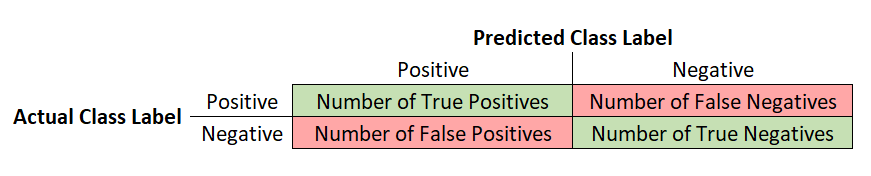
The confusion matrix is typically arranged in a square matrix format, with rows representing the actual class labels and columns representing the predicted class labels. For a binary classification problem, the confusion matrix consists of four cells:

True Positives (TP): The number of instances where the model correctly predicted the positive class.
True Negatives (TN): The number of instances where the model correctly predicted the negative class.
False Positives (FP): The number of instances where the model incorrectly predicted the positive class (Type I error).
False Negatives (FN): The number of instances where the model incorrectly predicted the negative class (Type II error).

The layout of a binary confusion matrix is as follows:

The confusion matrix can be extended to multi-class classification problems by expanding the number of rows and columns to match the number of classes. In this case, each cell represents the number of instances where the model predicted a certain class (column) and the actual class was another class (row).

By analyzing the confusion matrix, various performance metrics can be calculated, such as accuracy, precision, recall, F1 score, and specificity. These metrics provide a more comprehensive understanding of the model’s performance, helping identify areas where the model might be struggling or biased towards specific classes.

16. Regression

Regression is a type of supervised learning task where the objective is to predict a continuous numeric value, often referred to as the target variable or label, based on input features. Unlike classification, which deals with discrete categories, regression focuses on modelling the relationship between input features and a continuous output. The goal is to develop a model that can accurately predict the target variable for new, unseen data based on the patterns and relationships it has learned during the training process.

For example, consider a dataset containing information about houses, including features such as the size, age, and number of rooms, along with the corresponding selling price of each house. A regression model, such as linear regression or a decision tree regressor, can be trained on this dataset to predict the selling price of houses based on their features. The model learns the underlying relationship between the features and the house prices during the training process, enabling it to predict the price for new, unseen houses with similar features. In this scenario, the regression task involves estimating a continuous numeric value (house price) based on the input features (size, age, and number of rooms).

17. Linear Regression

Linear regression is a supervised learning algorithm. It is probably the simplest possible regression algorithm. Linear regression assumes a linear relationship between the input features and the target variable, meaning that the predicted output is a linear combination of the input features, weighted by the model’s parameters. Or in other words, linear functions are used to map the features to the label.

Linear regression is simple, interpretable, and computationally efficient, making it a popular choice for regression tasks with relatively small datasets or when a linear relationship between the input features and the target variable is expected.

One particularly good use for linear regression, is that due to its simplicity, it is a good starting point for beginning to learn about machine learning. It can be thought of as the “Hello World!” of machine learning.

18. Logistic Regression

Logistic regression is a supervised learning algorithm used for classification tasks, particularly binary classification, where the goal is to assign input data to one of two discrete categories or classes. Despite its name, logistic regression is a classification algorithm, not a regression algorithm. It works by modelling the probability of an input belonging to a certain class based on its features. Logistic regression assumes a linear relationship between the input features and the log-odds of the probability of belonging to the positive class, making it a generalized linear model.

To make predictions, logistic regression applies the logistic (or sigmoid) function to the linear combination of input features and the model’s parameters, converting the linear output into a probability value ranging from 0 to 1. The algorithm aims to find the optimal parameters, or weights, that minimize the difference between the predicted probabilities and the actual class labels in the dataset. This is typically achieved using methods such as maximum likelihood estimation or gradient descent. Logistic regression is widely used for binary classification tasks due to its simplicity, interpretability, and efficiency in handling large datasets with a mix of continuous and categorical input features.

19. Naive Bayes

Naive Bayes is a family of probabilistic supervised learning algorithms used for classification tasks, particularly in situations where the dataset has a large number of features or when the training data is limited. Naive Bayes classifiers are based on Bayes’ theorem, which describes the relationship between the conditional and marginal probabilities of events. These classifiers are called “naive” because they make the strong assumption that the input features are conditionally independent given the class label, which simplifies the computation of probabilities.

Despite this simplifying assumption, Naive Bayes classifiers often perform well in practice, particularly in text classification tasks such as spam filtering or sentiment analysis. The training process involves calculating the probabilities of each class and the conditional probabilities of each feature given each class using the training data. When making predictions, Naive Bayes classifiers compute the posterior probability of each class given the input features and assign the input to the class with the highest probability. These classifiers are computationally efficient, easy to implement, and capable of handling large feature spaces, making them a popular choice for a variety of classification tasks.

20. Support Vector Machine (SVM)

Support Vector Machines (SVM) is a powerful and widely used supervised machine learning algorithm. The algorithm aims to classify data by finding the optimal decision boundary or hyperplane that maximally separates the data into different classes. This hyperplane is determined by the points closest to it, called support vectors. SVMs can handle linearly separable as well as non-linearly separable data by projecting the data into a higher dimensional space where it becomes linearly separable.

The SVM algorithm can be used for regression (then it’s called Support Vector Regression or SVR), but is more typically used for classification. For classification, SVM tries to find the hyperplane that maximizes the margin, which is the distance between the hyperplane and the closest points from each class. This makes SVMs a robust algorithm that can handle noise and outliers in the data. In addition, SVMs can be extended to handle multi-class classification problems by using one-vs-one or one-vs-all approaches.

One of the strengths of SVMs is their ability to use kernel methods to map the data to a higher dimensional space, where it becomes linearly separable. SVMs have been successfully used in various fields, such as image classification, text classification, and bioinformatics. However, SVMs can be computationally expensive for large datasets and can suffer from overfitting if the hyperparameters are not properly tuned.

21. Kernel Method, 22. Kernel Function, and 23. Kernel Trick

The kernel method is a popular technique used in machine learning for various tasks such as classification, regression, and clustering. It is particularly useful for working with nonlinear data since it allows the use of linear algorithms by transforming the data into a higher-dimensional space.

By mapping (not linearly separable) data points to a higher-dimensional feature space where they can be linearly separated, we can use linear decision boundaries to correctly classify the data points. The kernel method enables us to solve complex problems that cannot be solved in the original input space with linear separation boundaries.

The kernel function is the core of the kernel method. It takes two inputs and returns a similarity measure between them. The function must be symmetric, positive semi-definite, and satisfy the Mercer condition. The most commonly used kernel functions are the linear kernel, polynomial kernel, Gaussian kernel, and sigmoid kernel.

The kernel trick is a technique that allows the kernel method to efficiently perform computations in the higher-dimensional feature space without explicitly computing the coordinates of the data in that space. This is done by representing the data as dot products in the feature space, which can be computed efficiently using the kernel function.

To illustrate the kernel method and kernel trick, consider the case of SVMs. They work by finding the hyperplane that maximally separates the two classes in the feature space. Using the kernel trick, the SVM can implicitly transform the data into a higher-dimensional space without actually computing the coordinates in that space. This allows the SVM to work efficiently even in high-dimensional feature spaces.

In summary, the kernel method is a powerful technique for working with nonlinear data in machine learning. The kernel function is the key to this technique, providing a similarity measure between data points. The kernel trick is a clever way of computing in the higher-dimensional feature space without actually computing the coordinates, making the method efficient and practical.

24. Hard margin classifier

A hard margin classifier is a type of linear classifier that attempts to find a hyperplane that perfectly separates two classes of data. This is what the most basic approach to SVMs does. The goal of a hard margin classifier is to find a decision boundary that correctly classifies all the training examples with no errors. This means that there is no overlap between the two classes, and the hyperplane is as far away from the nearest data point as possible. In other words, the margin between the two classes is maximized. However, this approach is often too rigid and unrealistic in real-world applications, as there is almost always some noise or outliers in the data, making it difficult or impossible to find a perfect separation.

To construct a hard margin classifier, the data must be linearly separable, meaning that there exists a hyperplane that can separate the data into two classes. The classifier tries to maximize the margin between the hyperplane and the closest points from each class, subject to the constraint that all points must be classified correctly. The optimization problem can be formulated as a quadratic programming problem, which can be solved using various optimization techniques. However, if the data is not linearly separable, the optimization problem is infeasible, and a soft margin classifier, which allows some misclassifications, may be more appropriate.

25. Soft margin classifier

A soft margin classifier is a type of linear classifier in machine learning that allows for some misclassifications in the training data. Unlike the hard margin classifier, the soft margin classifier can handle non-linearly separable data, where there is no hyperplane that can perfectly separate the classes. The goal of a soft margin classifier is to find a hyperplane that separates the classes as best as possible while allowing some misclassifications. This is done by introducing a penalty term that punishes the classifier for misclassifying data points, and the penalty is minimized along with the margin.

To construct a soft margin classifier, the data is first transformed into a higher-dimensional space where a linear decision boundary may be more feasible. The optimization problem is then formulated as minimizing the margin and the penalty term simultaneously, subject to the constraint that all points must be classified correctly within a certain margin. The penalty term is typically the sum of the distances from the misclassified points to the margin, and the regularization parameter controls the trade-off between maximizing the margin and minimizing the penalty. The optimization problem can be solved using various techniques such as quadratic programming, gradient descent, or kernel methods.

26. Radial Basis Function (RBF)

Radial Basis Function (RBF) is a function, whose value depends on the distance from origin, or some predetermined point (called center or centroid). RBFs are used as kernel functions in machine learning to transform the input data into a higher-dimensional space where it can be more easily separated. The RBF computes the similarity between a given input data point and a set of pre-defined reference points called centroids. The output of the kernel function is then used as the input for a linear model, which can be used for classification or regression tasks. The RBF kernel is defined as a radial function of (usually) the Euclidean distance between the input data point and the centroid. The RBF kernel has a smooth and continuous shape, which makes it well-suited for a variety of applications.

RBF networks are widely used in many applications such as image recognition, speech recognition, and financial forecasting. They have the advantage of being able to approximate any continuous function to any desired accuracy, making them very flexible and powerful. RBF networks are also computationally efficient, as they require only a small number of parameters compared to other neural network models. However, RBF networks can be sensitive to the choice of the kernel function and the number and location of the centroids, which can affect the performance of the model. Thus, careful tuning and selection of these parameters is important for achieving optimal performance.

27. K-Nearest Neighbors (KNN)

K-Nearest Neighbors (KNN) is a non-parametric, instance-based supervised learning algorithm used for both classification and regression tasks. KNN is considered non-parametric because it makes no explicit assumptions about the underlying distribution of the data, and it is instance-based because it stores the entire training dataset in memory rather than learning a model from the data. KNN operates on the principle of similarity, assuming that data points that are close to each other in feature space share similar characteristics and should belong to the same class or have similar target values.

In the classification context, when given a new, unseen data point, KNN finds the K training data points that are closest to the new data point based on a chosen distance metric, such as Euclidean or Manhattan distance. The algorithm then assigns the most common class label among the K nearest neighbors to the new data point. In the case of regression, KNN predicts the target value for the new data point by averaging the target values of its K nearest neighbors.

One of the main advantages of KNN is its simplicity and ease of implementation. However, it has some drawbacks, such as high computational cost during prediction due to the need to compute distances to all training data points, sensitivity to the choice of distance metric and the value of K, and poor performance with high-dimensional data or data with irrelevant features. To address these issues, practitioners often employ techniques such as feature scaling, dimensionality reduction, and efficient search algorithms to improve the performance of KNN in specific problem domains.

28. Decision Tree

Decision trees are a family of supervised learning algorithms used for both classification and regression tasks. A decision tree is a hierarchical data structure that represents a set of decisions and their corresponding outcomes. It consists of nodes, where each node represents a decision based on a specific feature, and branches, which represent the possible outcomes of that decision. The terminal nodes, also known as leaves, represent the final prediction or class label in classification tasks or the predicted target value in regression tasks.

During the training process, the decision tree algorithm recursively splits the dataset based on the feature that provides the best separation of the target variable, according to a chosen criterion. In classification tasks, commonly used criteria are Gini impurity and information gain, while in regression tasks, mean squared error or mean absolute error are typically used. The process continues until a stopping condition is met, such as reaching a maximum tree depth or a minimum number of samples in a leaf.

Decision trees are popular for their simplicity, interpretability, and ability to handle both categorical and continuous input features. However, they can be prone to overfitting, especially when the tree is deep and complex. To mitigate this issue, practitioners often use techniques such as pruning or limiting the tree depth to create simpler trees that generalize better to unseen data. Additionally, decision trees can be combined in ensemble methods, such as random forests or gradient boosting machines, to improve predictive performance and robustness.

29. Instance-Based Learning

Instance-based learning is a type of machine learning algorithm that learns by comparing new input data to the existing training instances. The training data consists of labeled examples, where each example is a pair of input features and an associated output label. During training, the algorithm simply memorizes the training examples, storing them in memory for future use. When presented with a new input instance, the algorithm finds the most similar training example(s) and predicts the output label based on the labels of those examples. The similarity between instances is usually measured using some distance metric, such as Euclidean distance or cosine similarity.

Instance-based learning has several advantages over other types of machine learning algorithms. First, it is very simple and easy to understand, requiring little to no parameter tuning. Second, it is well-suited to handling noisy or complex data, since it can rely on the training examples to handle edge cases. Finally, instance-based learning can be used for both classification and regression tasks, making it a versatile approach. However, it can also be computationally expensive, since it requires searching through the entire training dataset for each new instance.

30. Decision boundary

A decision boundary is a hypothetical boundary that separates different classes or clusters of data points in a feature space. It is a critical component of classification algorithms as it determines how data points are assigned to different classes. The decision boundary is often represented as a hyperplane in a high-dimensional feature space, but it can take other forms in different contexts.

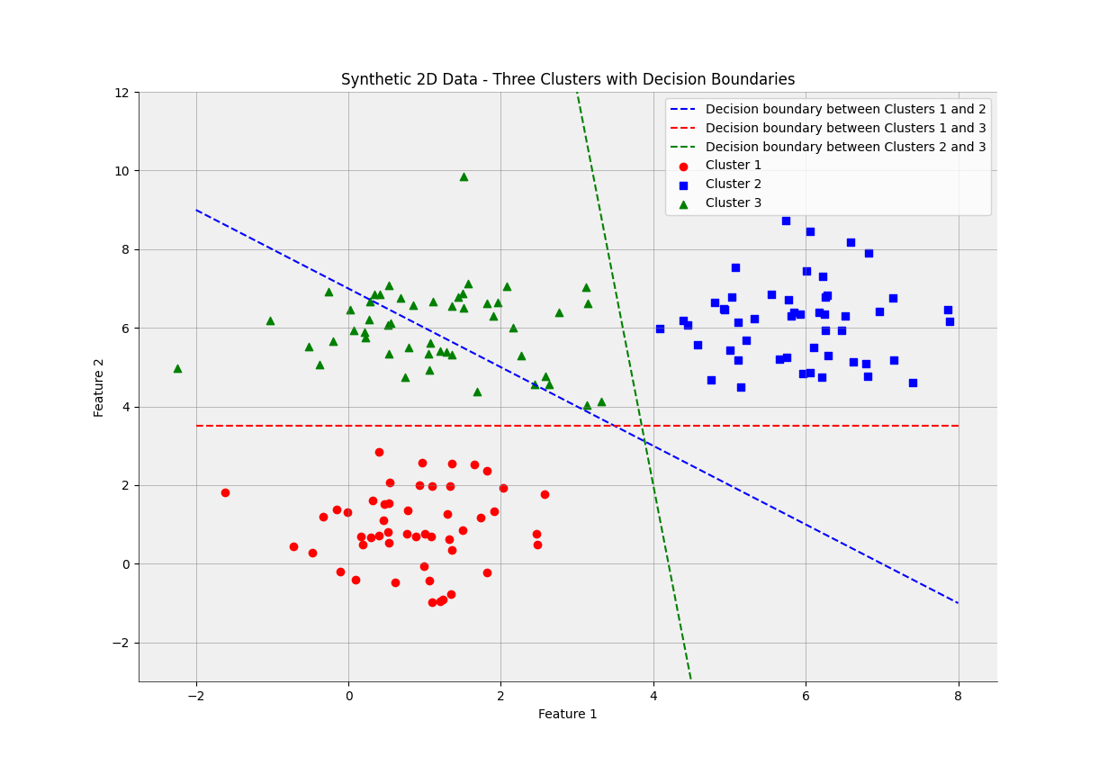
In this Figure, you can see three clusters of data points in a 2-dimensional feature space, separated from each other by linear decision boundaries.

The goal of a classification algorithm is to learn a decision boundary that can accurately separate the data points into their respective classes. This is achieved through a training process that involves adjusting the parameters of the model to minimize the error between the predicted class and the actual class of the data points. Once the decision boundary has been learned, the model can be used to predict the class of new data points based on which side of the boundary they lie.

In summary, a decision boundary is a boundary that separates different classes or clusters of data points in a feature space. It is a critical component of classification algorithms, and its accuracy is essential for the success of the model.

31. Overlapping Data

Overlapping data refers to instances where the feature values of different classes or categories are not clearly separated in the feature space. This overlap can make it challenging for machine learning algorithms to accurately classify or predict outcomes, as it is more difficult to identify a clear boundary between classes. Overlapping data is common in real-world problems, where noise, outliers, or complex relationships between features can lead to a mix of data points from various classes in the same region of the feature space.

Addressing overlapping data often involves applying advanced techniques to improve the performance of machine learning models. These techniques might include feature engineering, which seeks to create new, more discriminative features; feature selection, which aims to remove irrelevant or redundant features that contribute to the overlap; or dimensionality reduction, which can help uncover hidden patterns or structures in the data. Additionally, ensemble methods like bagging and boosting can increase the robustness and accuracy of models when dealing with overlapping data by combining the predictions of multiple base learners.

32. Empirical Risk, and 33. Empirical Risk Minimization (ERM)

Empirical risk is a measure of how well a machine learning model performs on a given set of training data. It is defined as the average loss over the training dataset. The goal of machine learning is to find a model that minimizes the empirical risk, so that it can make accurate predictions on new, unseen data.

Empirical Risk Minimization (ERM) is the name of the common approach in machine for finding the model that minimizes the empirical risk. The basic idea behind ERM is to train the model on a training set of labeled data by adjusting its parameters so that the empirical risk is minimized. Once the model is trained, it can be used to make predictions on new, unseen data.

The effectiveness of ERM depends on several factors, including the choice of the loss function, the capacity of the model, and the size and quality of the training data. The choice of loss function should be appropriate for the problem at hand, and the capacity of the model should be sufficient to capture the underlying patterns in the data without overfitting.

Despite its simplicity, ERM has been shown to be a powerful method for solving a wide range of machine learning problems and is widely used in practice.

34. Ensemble Learning (also known as Ensemble methods)

Ensemble learning is a technique used in machine learning to combine multiple models to improve the accuracy and robustness of predictions. Rather than relying on a single model, ensemble learning involves training multiple models on the same data and then combining their predictions to produce a final output. This approach can help reduce the risk of overfitting and improve the generalization performance of the model.

Ensemble learning can take different forms, such as bagging, boosting, and stacking.

Ensemble learning has been successfully applied in many machine learning tasks, including image and speech recognition, natural language processing, and anomaly detection, among others.

35. Bagging

Bagging (Bootstrap Aggregation) is a machine learning technique that involves building multiple models on random subsets of the training data, and then combining their predictions to obtain a final output. The random subsets of the training data are created by sampling the data with replacement, which means that some instances may appear multiple times in the same subset, while others may not appear at all. Bagging can be applied to a wide range of machine learning algorithms, including decision trees, neural networks, and support vector machines, and can help to reduce the variance of the model and prevent overfitting.

36. Boosting

Boosting is an ensemble learning technique in machine learning that combines multiple weak learners, typically decision trees, to create a strong classifier or regressor. The core idea behind boosting is to iteratively train weak learners, each of which focuses on correcting the mistakes made by the previous ones. By assigning higher weights to misclassified instances or increasing their importance, boosting forces the subsequent learners to concentrate on the more challenging examples. The final model is a weighted combination of the weak learners, producing more accurate predictions or classifications than any individual learner. Popular boosting algorithms include AdaBoost, Gradient Boosting, XGBoost, LightGBM, and CatBoost.

37. Gradient Boosting

Gradient Boosting is a powerful ensemble learning technique that builds a strong predictive model by combining multiple weak learners, typically decision trees, in a sequential manner. The main idea behind gradient boosting is to iteratively add weak learners to the ensemble, with each learner focusing on minimizing the residual errors or the difference between the true values and the predicted values from the previous ensemble model. This process helps the model improve its predictive performance over time by gradually reducing the overall error.

In gradient boosting, the weak learners are trained using the negative gradient of the loss function (hence the name “gradient boosting”) with respect to the model’s predictions. This approach enables gradient boosting to be applied to a wide range of loss functions and makes it suitable for both classification and regression tasks. At each iteration, a new weak learner is added to the ensemble, and its contribution is determined by optimizing the loss function for the entire ensemble. The final model is the sum of the weak learners, producing more accurate predictions than any individual learner.

38. AdaBoost (Adaptive Boosting)

The key idea behind AdaBoost is to train a series of weak classifiers (usually decision stumps, which are single-level decision trees) on the training data, where each classifier aims to correct the mistakes of its predecessor. During each iteration, AdaBoost assigns weights to the training instances, increasing the weights of misclassified instances and decreasing the weights of correctly classified instances. This process ensures that the subsequent weak classifiers pay more attention to the more challenging instances, effectively learning from the mistakes of previous classifiers.

The final strong classifier is a weighted majority vote of the weak classifiers, where the contribution of each weak classifier is determined by its classification accuracy on the weighted training data. The more accurate a weak classifier is, the higher its weight in the final ensemble.

AdaBoost is highly effective in a variety of classification tasks, including binary and multi-class problems. It is computationally efficient and often requires less hyperparameter tuning compared to other boosting algorithms. However, AdaBoost can be sensitive to noise and outliers in the data, which may result in overfitting or reduced performance.

39. XGBoost (eXtreme Gradient Boosting)

XGBoost is an open-source, scalable, and efficient machine learning library that implements the gradient boosted decision tree algorithm. It is designed to be highly efficient and flexible, providing parallel tree boosting and handling sparse data effectively. XGBoost is known for its speed and high-performance, often achieving better results than other gradient boosting techniques. It includes built-in regularization to prevent overfitting, as well as various hyperparameters for tuning the model for optimal performance.

40. LightGBM (Light Gradient Boosting Machine)

LightGBM is another open-source, gradient boosting framework developed by Microsoft. It is designed to be efficient and scalable for large datasets and high-dimensional data. LightGBM differs from other gradient boosting techniques by using a novel tree-growing method called Gradient-based One-Side Sampling (GOSS) and Exclusive Feature Bundling (EFB). GOSS focuses on selecting the most informative samples for tree growth, while EFB reduces the number of features by bundling exclusive features together. This results in faster training and reduced memory usage without compromising accuracy.

41. CatBoost (Categorical Boosting)

CatBoost is an open-source gradient boosting library developed by Yandex that is specifically designed for handling categorical features. It provides an efficient and accurate way to deal with categorical variables without the need for manual preprocessing such as one-hot encoding. CatBoost uses a combination of ordered boosting and oblivious trees to improve performance and reduce overfitting. It also includes various regularization techniques and supports GPU acceleration for faster training. CatBoost is known for its robust handling of categorical data and high accuracy in a variety of tasks, including classification and regression problems.

42. Stacking

Stacking, also known as stacked generalization, is a machine learning technique that involves combining multiple base models and training a meta-model on their predictions to obtain a final output. Unlike bagging and boosting, which focus on improving the performance of a single model, stacking aims to leverage the strengths of different models by combining them in a meaningful way. The base models can be trained on different subsets of the training data or use different algorithms, and the meta-model can be trained on the outputs of the base models to make a final prediction. Stacking can be a powerful technique for improving the performance of machine learning models, but it can also be more complex and time-consuming than other techniques.

43. Random Forest

Random forests are an ensemble learning method in machine learning that combines multiple decision trees to improve prediction accuracy and prevent overfitting. They operate by constructing numerous decision trees during the training phase and outputting the class or regression value that is the mode or mean of the individual tree predictions, respectively. This approach leverages the wisdom of the crowd, where the aggregated predictions from multiple trees yield better results than any single tree.

The random forest algorithm introduces randomness in two ways: bootstrapping the dataset and selecting a random subset of features at each split.

Bootsrapping: During the tree construction, the algorithm takes a random sample of the training data with replacement, which forms a bootstrap dataset for each tree.

Selecting a random subset of features: Additionally, at each split, the algorithm randomly selects a subset of features to consider for the best split, rather than evaluating all the features. These randomization techniques help to reduce correlation among the individual trees, making the ensemble more robust and accurate.

Random forests are popular for their versatility, handling both classification and regression tasks effectively. They can handle missing data, are robust to outliers, and provide variable importance rankings. Furthermore, they often require minimal parameter tuning and perform well with default settings. However, random forests can be computationally expensive, especially with large datasets and a high number of trees, which can lead to slower training and prediction times.

44. Ensemble Size

Ensemble size is a hyperparameter, that refers to the number of individual models that are combined to form an ensemble in machine learning. In general, larger ensembles tend to perform better than smaller ensembles, up to a point, where adding more models may result in diminishing returns or even overfitting. The optimal ensemble size depends on various factors, such as the complexity of the problem, the diversity of the models, and the available computational resources. Ensemble size can be controlled by adjusting the number of base models in bagging and boosting, or by setting the number of folds in cross-validation. In practice, ensemble size is often determined empirically by evaluating the performance of the ensemble on a validation set or through cross-validation.

45. Multi-task Learning

Multi-task learning is a machine learning technique that allows multiple related tasks to be learned simultaneously using a single model. In traditional machine learning, a separate model is trained for each task, but with multi-task learning, a single model is trained to perform multiple tasks. This approach can improve the performance of the model on each task, particularly when the tasks are related and share underlying structure. For example, in natural language processing, multi-task learning can help a model perform multiple tasks such as sentiment analysis, named entity recognition, and part-of-speech tagging more accurately by sharing information learned across these tasks.

The key challenge in multi-task learning is designing a shared representation that captures the commonalities between the tasks while still allowing the model to specialize for each individual task. This is typically done by combining multiple loss functions that correspond to each task, with a weighting scheme that allows the model to balance its attention between the tasks. Additionally, the architecture of the model can be designed to include shared layers that capture the common features between tasks, as well as task-specific layers that allow the model to specialize for each task. Overall, multi-task learning is a powerful technique that can improve the efficiency and effectiveness of machine learning models across a wide range of applications.

46. Overfitting and 47. Underfitting

Overfitting and underfitting are two common issues that occur in machine learning when a model does not generalize well to new, unseen data.

Overfitting:

Overfitting occurs when a model learns the training data too well, including the noise and random fluctuations present in the data. This results in a model that performs exceptionally well on the training data but poorly on new, unseen data. The model becomes too complex and is unable to generalize the underlying patterns or relationships in the data.

Example: Imagine you are training a model to predict house prices based on various features like the size, location, and age of the property. If the model is overfitting, it may memorize the prices of the houses in the training dataset, even capturing minor fluctuations and noise that are not representative of the general market trend. As a result, when presented with new data, the model will make inaccurate predictions, as it has not learned the true underlying relationship between the features and house prices.

Overfitting is generally easy to detect from the learning curve.

Underfitting:

Underfitting occurs when a model is too simple to capture the underlying patterns or relationships between the features and the target variable in the data. The model fails to learn the true structure of the data and performs poorly on both the training data and new, unseen data. This usually happens when the model lacks sufficient complexity or has not been trained long enough.

Example: Continuing with the house price prediction example, if the model is underfitting, it may only consider one feature, such as the size of the property, to predict the price. This simplistic approach fails to account for other important factors like location and age, leading to inaccurate predictions for both the training and test data, as the model has not captured the true relationship between all relevant features and house prices.

To achieve a good balance between overfitting and underfitting, it is crucial to select an appropriate model complexity, use regularization techniques, and validate the model using techniques like cross-validation or splitting the data into training, validation, and test sets.

48. Hyperparameters and 49. Hyperparameter tuning

Hyperparameters are the adjustable parameters or settings of a machine learning model that control the learning process and influence the model’s performance. Unlike model parameters, which are learned by the model during training (e.g., weights and biases in a neural network), hyperparameters are set by the practitioner before training starts. They play a crucial role in determining the model’s ability to generalize to new data.

Some examples of hyperparameters include:

Learning rate in gradient descent optimization.
Regularization parameter (alpha or lambda) in Lasso, Ridge, or Elastic Net regression.
Number of trees and maximum depth in Random Forest or Gradient Boosting algorithms.
Number of hidden layers and neurons in a neural network.
Kernel function and regularization parameter in Support Vector Machines.

Hyperparameter tuning, also known as hyperparameter optimization, is the process of finding the optimal set of hyperparameter values that yield the best performance for a machine learning model. The goal is to find the right balance between model complexity and generalization ability, minimizing the risk of overfitting or underfitting.

There are several techniques for hyperparameter tuning, including:

Grid Search: This method involves exhaustively searching through a predefined set of hyperparameter values and selecting the combination that results in the best model performance, usually measured by cross-validated scores or a held-out validation set.
Random Search: Instead of searching through all possible combinations, random search samples hyperparameter values from a predefined distribution. This method can be more efficient than grid search, as it allows for better exploration of the hyperparameter space with fewer iterations.
Bayesian Optimization: This technique uses a probabilistic model to guide the search for optimal hyperparameters. It takes into account the past evaluation results to build a surrogate model, which is then used to decide the next set of hyperparameters to evaluate. This allows for more intelligent exploration of the hyperparameter space and can converge to the optimal values faster than grid or random search.

Hyperparameter tuning is an essential step in the model development process, as selecting the right hyperparameters can significantly improve a model’s performance and ability to generalize to new data.

50. Regularization

Regularization is a technique used in machine learning to prevent overfitting, improve model generalization, and, in some cases, handle multicollinearity. It works by adding a penalty term to the model’s objective function (also known as cost or loss function), which discourages the model from fitting the training data too closely.

The purpose of regularization is to reduce the complexity of the model by penalizing certain model parameters if they have a large magnitude. By doing so, the model becomes less sensitive to individual data points in the training set and is better able to generalize to new, unseen data.

Lasso Regression, Ridge Regression, and Elastic Net are examples of regularization techniques used in linear regression models to prevent overfitting, improve model generalization, and handle multicollinearity.

51. Lasso Regression (Least Absolute Shrinkage and Selection Operator)

Lasso Regression adds an L1 regularization term to the linear regression cost function, which is the absolute value of the coefficients multiplied by a regularization parameter (lambda or alpha). This technique not only helps prevent overfitting but also encourages sparsity in the model by shrinking some of the coefficients to zero. As a result, Lasso Regression can also perform feature selection, making the model more interpretable by retaining only the most relevant features.

Cost Function: Cost = Mean Squared Error + (alpha * |w|)

52. Ridge Regression (L2 Regularization)

Ridge Regression introduces an L2 regularization term to the linear regression cost function, which is the squared value of the coefficients multiplied by a regularization parameter (lambda or alpha). This technique helps prevent overfitting by penalizing large coefficients, effectively reducing their impact on the model. Unlike Lasso Regression, Ridge Regression does not force coefficients to zero but shrinks them towards zero, retaining all features in the model.

Cost Function: Cost = Mean Squared Error + (alpha * w²)

53. Elastic Net

Elastic Net is a combination of both Lasso and Ridge Regression techniques, incorporating both L1 and L2 regularization terms into the cost function. It provides a balance between Lasso’s sparsity and feature selection properties and Ridge’s ability to handle multicollinearity. Elastic Net includes an additional hyperparameter, called the mixing parameter (rho), which determines the relative weight of the L1 and L2 regularization terms.

Cost Function: Cost = Mean Squared Error + (alpha * (rho * |w| + (1 – rho) * w²))

In summary, Lasso, Ridge, and Elastic Net are regularization techniques that add penalties to the linear regression cost function to prevent overfitting and improve generalization. Lasso encourages sparsity and performs feature selection, Ridge handles multicollinearity, and Elastic Net combines the properties of both Lasso and Ridge, providing a balanced approach.