Machine Learning Glossary - 50+ Concepts You Should Know

This is a glossary of more than 50 terms in the fields of Artificial Intelligence (AI) and Machine Learning (ML). These terms cover the fields very broadly. Use this glossary to gain introductory knowledge of the field, or use CTRL + F to read the description only for the concepts you are interested in!

I have structured the terms in categories that are closely related in the hopes that it will make it easier for you to grasp the big picture! I also added links from different terms and concepts to each other, so you can quickly jump between them!

Also, check out our glossaries of terms and concepts for more specific subfields under Machine Learning and Artificial Intelligence:

Without further ado, let’s get onto the list!

1. Artificial Intelligence (AI) and 2. Machine learning (ML)

Artificial Intelligence (AI) and Machine Learning (ML) are closely related fields in computer science that deal with creating intelligent systems capable of performing tasks without explicit human programming.

Artificial Intelligence (AI) refers to the broader concept of creating machines or systems that can simulate human-like intelligence, reasoning, learning, and problem-solving. The primary goal of AI is to develop systems that can understand, interpret, and respond to their environment, and exhibit human-like cognitive abilities such as decision-making, language understanding, and pattern recognition.

Machine Learning (ML), a subset of AI, is the process by which computers learn from data to improve their performance on a specific task. Instead of being explicitly programmed with rules or algorithms, ML models are trained on large datasets to identify patterns, make predictions, and recognize complex relationships. This learning process usually involves using statistical techniques and optimization algorithms to minimize errors in the model’s predictions, enabling the model to improve over time as it is exposed to more data.

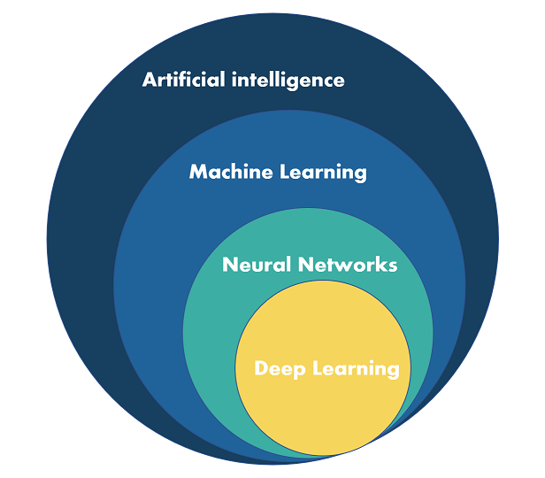
In essence, Machine Learning is one of the key methods used to achieve Artificial Intelligence. While AI encompasses a wide range of techniques and approaches to create intelligent systems, ML focuses on the data-driven aspect of building AI systems that can learn and adapt over time. Other AI techniques and subfields include e.g. search algorithms, constraint solving and optimization, automated reasoning, theorem proving, decision making and planning.

In summary, AI is the broader field of developing intelligent systems, while ML is a specific approach within AI that focuses on creating systems that can learn from data. ML plays a crucial role in helping AI systems achieve human-like intelligence and adaptability.

3. Supervised Learning

Supervised learning is a type of machine learning where an algorithm learns to make predictions based on a set of labeled input-output pairs. In this process, the model is trained using a dataset that contains input data (known as features) along with the correct output (known as the label). The algorithm generalizes the relationship between the inputs and outputs to make accurate predictions on unseen data.

For example, consider the following cases:

Email spam filtering: In this application, a supervised learning algorithm learns to classify emails as spam or not spam. The training dataset contains numerous emails, each labeled as either spam or not spam. The algorithm learns to recognize patterns and features associated with spam emails, enabling it to predict whether a new, unseen email is spam or not.
Handwritten digit recognition: The algorithm is trained on a dataset of labeled images of handwritten digits, with each image containing a single digit from 0 to 9. The model learns to recognize the unique features of each digit, such as curves and lines, and can then correctly identify handwritten digits in new, unlabeled images.
Medical diagnosis: A supervised learning algorithm can be trained to diagnose diseases based on medical records. The training dataset consists of records with various patient attributes, such as age, weight, and symptoms, along with the corresponding diagnosis. The model learns the relationship between these attributes and the diagnosis, allowing it to predict the correct diagnosis for new patients based on their attributes.

In summary, supervised learning involves training an algorithm using labeled input-output pairs, allowing it to generalize the relationship between the inputs (features) and outputs (labels). This understanding enables the model to make accurate predictions on unseen data

Supervised learning has widespread applications across various industries, including healthcare, finance, and natural language processing, to name a few. By employing supervised learning techniques, organizations can harness the power of data to solve complex problems, enhance decision-making processes, and create innovative solutions for real-world challenges.

Psst. You should also check out our more comprehensive glossary about Supervised Learning.

4. Unsupervised Learning

Unsupervised learning is a type of machine learning where an algorithm learns to identify patterns or structures in data without the guidance of labeled input-output pairs. In this approach, the model works with unlabeled data and focuses on discovering underlying patterns, grouping similar data points together, or reducing the dimensionality of the data.

Consider the following examples:

5. Clustering

In this application, an unsupervised learning algorithm groups similar data points together based on their features. For instance, a company may use clustering to segment customers based on their purchasing behavior, demographics, or preferences, without any prior knowledge of the number of segments or their characteristics. By identifying these customer groups, businesses can tailor marketing strategies to target each segment effectively.

6. Anomaly detection

Unsupervised learning algorithms can be employed to identify unusual or suspicious activities in data. For example, in credit card fraud detection, the model learns the normal patterns of transaction data and can then flag any transactions that significantly deviate from these patterns as potential fraud.

7. Dimensionality reduction

Techniques like Principal Component Analysis (PCA) help reduce the number of features in a dataset while retaining most of the original information. This process simplifies complex datasets, making it easier for other machine learning algorithms to process and analyze the data. For example, in image recognition tasks, dimensionality reduction can help remove noise and irrelevant features from the images, improving the efficiency and accuracy of subsequent models.

In summary, unsupervised learning involves working with unlabeled data to uncover hidden patterns, group similar data points, or simplify datasets. This approach plays a crucial role in various applications, such as customer segmentation, anomaly detection, and data preprocessing. Unsupervised learning enables organizations to extract valuable insights from large volumes of data without requiring labeled input-output pairs. By leveraging unsupervised learning techniques, businesses and researchers can uncover new relationships, identify previously unknown trends, and gain a deeper understanding of complex data, ultimately driving innovation and enhancing decision-making processes.

Psst. You could also check out our more comprehensive glossary about Unsupervised Learning.

8. Reinforcement Learning (RL)

Reinforcement Learning is a type of machine learning where an agent learns to make decisions by interacting with an environment. The agent takes actions, observes the resulting states and receives feedback in the form of rewards or penalties. The goal is to learn a policy, which is a mapping from states to actions, that maximizes the cumulative reward over time.

In RL, the agent and environment continually interact in a loop. The agent takes an action based on its current state, the environment responds by updating the state and providing a reward, and the agent learns from this feedback to improve its future actions. The agent’s learning is typically guided by algorithms like Q-learning or Proximal Policy Optimization.

Let’s look at a few examples to understand the concept of reinforcement learning better:

Playing games: In games like chess or Go, an RL agent learns to make strategic moves by playing against itself or other opponents. It receives a reward for winning and a penalty for losing. Through this process, the agent learns a policy that helps it choose the best moves given a particular game state.
Autonomous vehicles: RL agents can be used to control self-driving cars. The agent learns to navigate a car by observing its environment, making decisions about speed, direction, and when to brake or accelerate. Rewards are given for smooth, safe driving, while penalties are assigned for collisions or traffic violations.
Robot control: Reinforcement learning can be applied to teach robots how to perform tasks, such as grasping objects, walking, or flying. For example, a robotic arm learns to pick up objects by exploring different grasping techniques and receiving rewards for successful grasps while being penalized for dropping objects or failing to pick them up. Over time, the RL agent refines its policy to maximize the rewards, resulting in improved performance and task efficiency.
Financial trading: In the world of finance, RL agents can be used to optimize trading strategies. The agent learns to make buy or sell decisions based on market data, attempting to maximize the overall profit. Rewards are given for profitable trades, while penalties are applied for losses. As the agent continues to learn, it becomes better at identifying patterns and making informed trading decisions.
Healthcare: RL can be applied in healthcare to personalize treatment plans for patients. The agent learns to recommend treatments based on a patient’s medical history, current symptoms, and other relevant factors. The agent receives rewards for improved patient outcomes and penalties for negative results. Over time, the RL agent develops a more refined policy that effectively tailors treatment plans for individual patients.

These examples demonstrate the versatility and potential of reinforcement learning across various domains. By enabling agents to learn from their experiences and improve their decision-making, RL has the potential to transform industries and solve complex problems.

Psst. You could also check out our more comprehensive glossary about Reinforcement Learning.

9. Deep Learning

Deep learning is a subfield of machine learning that focuses on training artificial neural networks (ANNs) to recognize patterns and make decisions. These networks, inspired by the human brain, consist of interconnected layers of nodes or neurons, which process and transmit information.

In deep learning, a neural network learns to identify patterns by adjusting the weights and biases of its connections. It uses a process called backpropagation to minimize the error between predicted and actual outputs. As the network trains on more data, it becomes better at recognizing patterns and making accurate predictions.

Here are some examples of deep learning applications:

Image recognition: Deep learning models, such as convolutional neural networks (CNNs), can identify and classify objects within images. For instance, they can detect and differentiate between cats, dogs, and other objects, making them valuable for applications like photo organization or surveillance systems.
Natural language processing: Recurrent neural networks (RNNs) and transformers are used in deep learning for understanding and generating human language. They can analyze text for sentiment, translate languages, and even generate human-like text, as seen in chatbots and language models like GPT-4.
Speech recognition: Deep learning models can convert spoken language into written text, allowing for applications like voice assistants, transcription services, and hands-free device control.
Autonomous vehicles: Deep learning helps self-driving cars perceive and navigate their environment by recognizing and interpreting street signs, traffic signals, pedestrians, and other vehicles.
Game playing: Deep learning models, like DeepMind’s AlphaGo, have demonstrated the ability to learn and master complex games such as Go and chess. These models use reinforcement learning, a type of deep learning, to explore and evaluate possible moves, continuously improving their strategies over time. This has resulted in AI systems that can defeat world champions and achieve superhuman performance in these games.
Medical diagnosis: Deep learning models can analyze medical images, such as X-rays, MRI scans, and CT scans, to detect and diagnose diseases like cancer, diabetes, and Alzheimer’s. These models can help healthcare professionals make more accurate and timely diagnoses, improving patient outcomes.
Recommender systems: Many online platforms, such as Netflix, Amazon, and Spotify, use deep learning algorithms to analyze user preferences and deliver personalized content recommendations. These models can predict which movies, products, or songs a user is likely to enjoy based on their browsing and consumption history.

In summary, deep learning is a powerful technique that allows artificial neural networks to learn complex patterns and make decisions based on large amounts of data. With applications spanning numerous industries and domains, deep learning continues to drive advancements in artificial intelligence and transform the way we interact with technology.

Psst. You could also check out our more comprehensive glossary about Deep Learning.

10. Semi-Supervised Learning

Semi-supervised learning is a machine learning approach that combines labeled and unlabeled data to improve the performance of a model. In traditional supervised learning, a model is trained using only labeled data, where each input is paired with a corresponding output. However, in many real-world scenarios, labeled data can be scarce and expensive to obtain. Semi-supervised learning can help overcome this limitation by leveraging the abundance of unlabeled data that is often available. By combining the labeled and unlabeled data, semi-supervised learning can improve the model’s performance by enabling it to learn from more data than it would be able to otherwise.

The key challenge in semi-supervised learning is to effectively utilize the unlabeled data to improve the model’s performance. This can be done by incorporating a regularization term in the objective function that encourages the model to generate similar outputs for similar inputs, even when those inputs are unlabeled. Alternatively, the model can be designed to explicitly capture the structure of the data, allowing it to generalize better to new, unseen inputs. Overall, semi-supervised learning is a powerful approach that can improve the performance of machine learning models when labeled data is scarce, expensive, or difficult to obtain.

11. Dataset

In the context of machine learning, a dataset is a collection of data points used to train, validate, or evaluate a machine learning model. Each data point in the dataset represents a single observation or example and is characterized by multiple features, which are individual measurable properties or characteristics of that observation. In supervised learning, data points also have associated labels, which are the correct answers or outcomes that the model aims to predict.

12. Datapoint

A data point is a single instance in the dataset. It can be a row in a table or an object with multiple attributes. Each data point contains a set of features and, in supervised learning, a corresponding label.

13. Feature

Features are the measurable properties or characteristics of a data point. They provide information about the data point and serve as input to the machine learning model. For example, in a dataset of houses, features might include the number of bedrooms, square footage, and location.

14. Label

Labels are the correct answers or outcomes associated with each data point in a supervised learning problem. They serve as the target variable that the machine learning model tries to predict. Using the house dataset example, if we want to predict the price of a house, the label would be the actual price of each house in the dataset.

Sometimes terms such as “labeled data” or “unlabeled data” are used. The former simply means datapoints, where the correct label of a datapoint is known, perhaps provided by a human analyzer, and the latter means datapoints, where the correct label is not known.

15. Training Dataset, 16. Validation Dataset, and 17. Test Dataset

In machine learning, the training, validation, and test datasets are distinct subsets of data used to develop, fine-tune, and evaluate a model’s performance. These datasets serve different purposes throughout the model development process, helping to prevent overfitting and ensure a model’s generalization to unseen data.

The training dataset is the largest portion of data used to teach the model the underlying patterns and relationships. Machine learning algorithms learn by adjusting their parameters based on the training data, optimizing their ability to make accurate predictions. For example, in a supervised learning task to identify handwritten digits, the training dataset would consist of labeled images of digits along with their corresponding numerical values.

The validation dataset is a separate (non-overlapping) subset of data used to tune the model’s hyperparameters and select the best model during the training process. By evaluating the model on the validation dataset, practitioners can identify and prevent overfitting, as well as determine the optimal model complexity. In the handwritten digit recognition example, the validation dataset might be used to compare different model architectures or tune hyperparameters such as learning rate and batch size.

The test dataset is an independent (again non-overlapping) subset of data reserved for evaluating the model’s final performance after training and hyperparameter tuning. The test dataset should not be used during the training or validation process, ensuring an unbiased assessment of the model’s ability to generalize to unseen data. In the digit recognition example, the test dataset would be used to measure the model’s accuracy in classifying previously unseen handwritten digits after training multiple models and choosing the best performing one in the validation step, providing an estimate of its real-world performance.

18. Imbalanced Dataset

In machine learning, an imbalanced dataset refers to a dataset in which the classes or categories are not equally represented. For example, in a binary classification problem, if one class accounts for only 10% of the total instances while the other accounts for 90%, then the dataset is said to be imbalanced. Imbalanced datasets are common in many real-world applications such as fraud detection, medical diagnosis, and anomaly detection.

Imbalanced datasets can pose a challenge to machine learning algorithms because they tend to favor the majority class, resulting in poor performance on the minority class. This is because the algorithm learns to optimize the overall accuracy, which can be achieved by simply predicting the majority class for every instance. To address this issue, various techniques have been developed to balance the dataset, such as undersampling the majority class, oversampling the minority class, or using a combination of both. Other approaches include generating synthetic data using techniques like SMOTE (Synthetic Minority Over-sampling Technique), or using cost-sensitive learning algorithms that penalize misclassification of the minority class more heavily than the majority class.

19. Big Data

Big Data in machine learning refers to the large-scale collection, storage, and analysis of vast and complex datasets that exceed the capabilities of traditional data processing systems. These datasets often possess high volume, velocity, and variety, presenting challenges in data management, processing, and extracting valuable insights. Machine learning algorithms leverage Big Data to build more accurate and sophisticated models by uncovering intricate patterns and relationships within the data, leading to better predictions and decision-making.

To handle Big Data, machine learning practitioners employ advanced technologies, such as distributed computing frameworks, parallel processing, and specialized hardware like GPUs. Techniques like data sampling, dimensionality reduction, and data compression are also used to reduce the scale and complexity of the data, making it more manageable for analysis. Machine learning models trained on Big Data can significantly improve performance across various domains, including natural language processing, image recognition, fraud detection, and recommendation systems.

20. Machine learning model (hypothesis space or predictor function space)

A machine learning model, also known as a hypothesis space or predictor function space, is a mathematical representation of the relationships between features and labels in a dataset. It is the core component of a machine learning system that helps in making predictions, classifications, or decisions based on input data. Machine learning models can take various forms, such as linear regression models, decision trees, or neural networks, depending on the type of problem and data being dealt with.

During the training process, a machine learning model learns patterns and relationships from the dataset by adjusting its parameters to minimize the difference between its predictions and the actual labels. This process often involves using optimization algorithms and loss functions to measure the discrepancy between the predicted and actual values. As the model iterates through the training process, it improves its ability to generalize from the training data and make accurate predictions on new, unseen data.

Once the model is trained, it can be used to make predictions on new data points by processing their features through the mathematical representation it has learned. The quality of a machine learning model’s predictions depends on factors such as the choice of algorithm, the quality and quantity of the training data, and the model’s ability to generalize from the training data to new, unseen situations. The main goal of a machine learning model is to accurately capture the underlying patterns and relationships in the data, enabling it to make reliable predictions on new data points.

21. Model Complexity and Model Capacity

Model complexity refers to the intricacy of a machine learning model’s architecture, encompassing the number of parameters, layers, and connections within it. Complex models possess a high degree of flexibility, allowing them to learn intricate patterns and representations from the input data. However, this complexity comes with a trade-off, as it can lead to overfitting when the model learns to capture noise or irrelevant patterns from the training data, resulting in poor generalization to unseen examples. Balancing model complexity is crucial in achieving a suitable trade-off between fitting the training data well and ensuring robust performance on new data.

Model capacity, on the other hand, represents the range of functions a machine learning model can potentially learn. A model with higher capacity has the ability to learn more complex relationships and patterns in the data, providing greater expressive power. This increased capacity can lead to better performance on complex tasks or when dealing with large, diverse datasets. However, like model complexity, a high-capacity model also risks overfitting if it becomes too specialized to the training data, hindering its ability to generalize effectively to new examples. Striking an optimal balance between model capacity and the risk of overfitting is essential for achieving the best possible performance on both training and testing data in machine learning applications.

22. Loss and 23. Loss Function

In the context of machine learning, loss is a measure of the difference between the predictions made by a machine learning model and the actual labels in the dataset. It quantifies the error or discrepancy between the model’s output and the correct answers, providing an indication of the model’s performance. A small loss indicates that the model is making accurate predictions, while a large loss suggests that the model’s predictions are far from the actual values.

A loss function, also known as a cost function or objective function, is a mathematical formula that calculates the loss for a given set of predictions and actual labels. The loss function serves as a guide for the machine learning model during the training process, helping it understand how well it is performing and which adjustments it needs to make to its parameters to improve its predictions. Different loss functions are used for different types of machine learning problems, such as mean squared error for regression tasks or cross-entropy loss for classification tasks.

Loss and loss functions are closely related concepts in machine learning. The loss function calculates the loss, providing a numerical representation of the model’s performance. By minimizing the loss during training, the model aims to improve its predictions and better capture the underlying patterns in the data. Optimization algorithms, such as gradient descent, are used in conjunction with loss functions to iteratively update the model’s parameters, reducing the loss and refining the model’s predictions. Ultimately, the choice of an appropriate loss function and the minimization of the loss are crucial steps in building accurate and reliable machine learning models.

24. Training Process

In supervised learning, the training process refers to fitting a machine learning model to a training dataset by minimizing the loss function, so that the model can make predictions or decisions based on new, unseen data. In reinforcement learning the training process involves the agent interacting with its environment, learning to maximize a reward signal (or minimize a penalty signal) while doing so.

Here are the key steps involved in a typical training process (specifically in supervised learning):

Data collection and preprocessing: The first step involves collecting and cleaning a large dataset that represents the problem you want the model to solve. This may involve data normalization, handling missing values, and feature extraction or selection.
Splitting data: The dataset is usually split into training, validation, and test sets. The training set is used to train the model, the validation set is used to tune hyperparameters and prevent overfitting, and the test set is used to evaluate the final model’s performance on unseen data.
Model selection: Choose an appropriate machine learning algorithm or model based on the problem type (e.g., classification, regression, clustering, etc.) and the nature of the data.
Model training: This is the actual training part. In this step the selected machine learning model is fitted to the training data. The internal parameters (e.g., weights and biases in a neural network) of the model are adjusted to minimize the loss function, by employing some optimization algorithm. This process is typically iterative and involves multiple passes through the training data.

25. Optimization

In the context of machine learning, optimization refers to the process of tuning the parameters of a model to minimize the loss (or maximizing a reward signal), thereby improving its performance on a given task. Optimization (in the form of minimizing the loss or maximizing the reward) is what is happening under the hood, when a ML model is being trained. When all goes well, optimization leads to the model learning the relationships between features and labels in the dataset. By iteratively adjusting the model’s parameters, optimization algorithms guide the model towards a solution that best fits the training data, resulting in more accurate predictions.

Various optimization algorithms exist, with gradient descent and its more advanced variants being some of the most popular. These algorithms work by computing the gradients of the loss function with respect to the model’s parameters and updating them accordingly. The gradients indicate the direction in which the parameters should be adjusted to minimize the loss. This process is repeated iteratively until a stopping criterion is met, such as reaching a predetermined number of iterations or observing no significant improvement in the loss. Ultimately, optimization is an essential aspect of machine learning, enabling models to learn from data and generalize to new, unseen situations.

Psst. You can also check out the Optimization Algorithms section from our Deep Learning Glossary.

26. Model Selection

Model selection refers to the process of choosing the best machine learning model for a specific problem or dataset. This process is crucial because different models can have varying performance on different tasks, and selecting the most suitable model can significantly impact the accuracy and reliability of predictions. Model selection involves evaluating and comparing different models, taking into consideration their complexity, accuracy, and generalization abilities, among other factors.

Model selection often starts with defining a set of candidate models or algorithms. These candidates can include different types of models, such as linear regression, decision trees, or neural networks, as well as variations of a single model type with different hyperparameters. The next step is to evaluate the performance of each candidate model using cross-validation techniques, such as a validation dataset. This helps to estimate the model’s performance on unseen data and assess its generalization capabilities.

After evaluating the candidate models, the one with the best performance on the validation data is selected. It’s important to note that the best model may not always be the one with the highest accuracy on the training data, as models with high training accuracy can sometimes overfit the data, leading to poor generalization on new data. Instead, the goal is to find a balance between model complexity and generalization ability, striking a balance between underfitting and overfitting.

In summary, model selection is a critical step in the machine learning process, as it helps identify the most suitable model for a given problem or dataset. By evaluating and comparing candidate models based on their performance on validation data, practitioners can select a model that achieves a balance between complexity and generalization ability, effectively mitigating the risks of underfitting and overfitting. Ultimately, proper model selection leads to more accurate and reliable predictions on new, unseen data.

27. Inference

Inference refers to the process of using a trained model to make predictions or decisions based on new data. After a model has been trained through a learning algorithm on a given dataset, it acquires the ability to recognize patterns and relationships within the data. Inference is the step where this knowledge is applied to draw conclusions or make predictions about new instances.

In simple terms, inference refers to feeding the features of a new datapoint into the trained machine learning model, and the model outputting its prediction.

28. Generalization

Generalization refers to a model’s ability to perform well on new, unseen data after being trained on a training dataset. A well-generalizing model can effectively apply the patterns and relationships it has learned from the training data to make accurate predictions or decisions on data it has never encountered before. Generalization is a critical aspect of machine learning, as it demonstrates the model’s capacity to adapt and provide meaningful insights beyond the specific instances it has seen during training.

Achieving good generalization depends on several factors, including the choice of the model, the quality and diversity of the training data, and the balance between model complexity and its capacity to learn underlying patterns. Overfitting and underfitting are common challenges in generalization. Overfitting occurs when a model learns the training data too well, including noise and irrelevant details, leading to poor performance on new data. Underfitting happens when a model is too simple to capture the underlying patterns in the data, resulting in suboptimal performance on both training and new data. The primary goal in machine learning is to find a balance between these two extremes, producing a model that can generalize effectively and provide reliable predictions on unseen data.

29. Overfitting

Overfitting occurs when a model learns the training data too well, capturing not only the underlying patterns but also the noise and irrelevant details. As a result, the model becomes highly accurate on the training data but performs poorly on new, unseen data. Overfitting often happens when a model is too complex, has too many parameters, or when the training data is limited or not diverse enough.

Overfitting can be detected by noticing, that the accuracy of the predictions is significantly higher on the training dataset, than on a separate validation dataset. Or similarly, it can be detected by noticing that the loss is significantly lower on the training dataset than on the validation dataset.

30. Overfitting Prevention

To prevent overfitting, several techniques can be employed during the training process. One popular approach is to split the dataset into three parts: training, validation, and testing sets. The model learns from the training data, while the validation set is used to fine-tune model parameters and monitor performance during training. The test set, which remains untouched until the final evaluation, provides an unbiased estimate of the model’s performance on unseen data. This partitioning is known as cross-validation, and it helps ensure that the model does not rely too heavily on the training data, promoting better generalization.

Another overfitting prevention technique is regularization, which involves adding a penalty term to the model’s loss function. This penalty term discourages the model from adopting overly complex solutions, thereby reducing the risk of overfitting.

31. Bias

Bias in machine learning refers to the presence of systematic errors in a model’s predictions due to underlying assumptions made during the model’s training process. It occurs when a model fails to capture the true complexity of the data, resulting in oversimplified predictions. High bias can cause underfitting, where the model does not perform well on either the training or the testing data, due to its inability to grasp the underlying patterns.

One primary source of bias is the lack of a diverse and representative dataset for training the model. If the training data is skewed or incomplete, the model learns to make predictions based on this limited information, leading to biased outcomes. For instance, a facial recognition system trained mostly on images of people with light skin tones may perform poorly on recognizing people with darker skin tones, exhibiting racial bias.

To mitigate bias in machine learning, practitioners must ensure the dataset is as diverse and representative as possible, and consider using techniques like cross-validation, ensemble methods, or regularization. It is crucial to continuously evaluate and update the model to improve its performance and fairness, thus reducing the impact of bias on the model’s predictions.

Bias can also refer to bias terms in neural networks.

32. Feature Engineering

Feature engineering is the process of transforming raw data into a more meaningful and useful format, creating new features, or improving existing ones to enhance the model’s performance. Feature engineering plays a critical role in building effective machine learning models, as it helps to extract valuable information from the data and ensure that the model can learn patterns and relationships more efficiently. Some types of Feature Engineering require domain expertise, while others do not.

Feature engineering involves various techniques, such as data cleaning, normalization, scaling, encoding categorical variables, and creating interaction features. Data cleaning typically involves handling missing values and removing outliers, while normalization and scaling help to bring features to a similar range, preventing some features from dominating others during the training process. Encoding categorical variables transforms non-numeric data into a numerical format that machine learning models can process. Creating interaction features involves combining two or more features to capture their combined effect on the target variable. By employing these techniques, practitioners can pre-process and transform the data to better represent the problem at hand, ultimately leading to improved model performance and more accurate predictions.

33. Regularization

Regularization is a technique used in machine learning to prevent overfitting by adding additional constraints or penalties to the model. The goal is to create a simpler model that is less likely to fit the noise in the training data and more likely to generalize well to new, unseen data.

34. Explicit regularization involves adding a penalty term to the objective function that the model is trying to minimize. The most common types of explicit regularization are L1 and L2 regularization. L1 regularization adds a penalty proportional to the absolute value of the model parameters, while L2 regularization adds a penalty proportional to the square of the parameters. The strength of the penalty is controlled by a hyperparameter, which is usually tuned using cross-validation.

35. Implicit regularization, on the other hand, refers to the effect of the learning algorithm itself on the model’s complexity. For example, algorithms such as gradient descent, which update the model parameters in small steps, tend to lead to smoother models and can act as an implicit regularization. Similarly, early stopping, which stops the training process when the model starts to overfit, can also act as an implicit regularization.

In practice, a combination of explicit and implicit regularization is often used to improve the generalization performance of machine learning models.

36. Early Stopping

Early stopping is another technique used to prevent overfitting in machine learning. During the training process, early stopping monitors the model’s performance on a validation dataset and terminates the training when the model’s performance on the validation data starts to degrade. This prevents the model from learning the noise in the training data and ensures that it generalizes better to new data.

37. Regularized Least Squares

In the context of machine learning, regularized least squares refers to using the MSE Loss as the loss function in a regression problem, while simultaneously incorporating regularization to further constrain the resulting solution.

Two popular forms of regularized least squares are Ridge Regression (L2 regularization) and Lasso Regression (L1 regularization). In Ridge Regression, the penalty term is proportional to the square of the model’s parameters, while in Lasso Regression, the penalty term is proportional to the absolute values of the parameters. Both techniques help to prevent overfitting by constraining the model’s parameters, but Lasso Regression has the added benefit of promoting sparsity, effectively performing feature selection by driving some parameter estimates to zero. By incorporating regularization into least squares, practitioners can build more robust models that generalize better to unseen data.

38. Dropout Regularization

Dropout regularization is a technique used in machine learning, particularly in deep learning, to prevent overfitting and improve model generalization. It involves randomly “dropping out” or deactivating a proportion of neurons in a neural network during training, ensuring that the model does not rely too heavily on any single neuron or connection. By temporarily removing neurons from the network, dropout forces the model to learn redundant representations, distributing the learned patterns more evenly across the network.

To implement dropout, a probability value (dropout rate) is set, indicating the likelihood of each neuron being deactivated during training. Commonly, dropout rates range from 0.2 to 0.5, depending on the complexity of the network and the dataset. During the forward pass, a neuron is deactivated with the set probability, and its outgoing connections are also removed. During the backward pass, gradients are not backpropagated through the deactivated neurons. It is important to note that dropout is only applied during training; during inference or testing, all neurons are active, and the network’s output is scaled based on the dropout rate to account for the additional active neurons. This ensures consistent performance and maintains the model’s overall behaviour.

39. Dropout Layer

A dropout layer is a specific layer in a neural network that implements dropout regularization. It is typically placed between consecutive layers, such as fully connected or convolutional layers, in the network. The dropout layer’s primary function is to deactivate a proportion of neurons from the previous layer during training, determined by the dropout rate, to prevent overfitting and promote better generalization. By introducing dropout layers in the architecture, the neural network learns more robust features and redundant representations, reducing its dependency on individual ne u rons. It is crucial to remember that dropout layers are only active during the training phase, while they have no impact during inference or testing, ensuring consistent model performance.

40. Hyperparameters

In machine learning, hyperparameters are parameters that are set prior to training a model and govern how the model is trained. These parameters cannot be learned during the training process and must be chosen manually by the user. Hyperparameters can significantly impact the performance of a model and therefore careful selection is essential. Some examples of hyperparameters include regularization strength, learning rate, batch size, number of layers, and number of neurons in each layer of a neural network.

The process of selecting hyperparameters can be time-consuming and requires a combination of knowledge, experimentation, and intuition. Hyperparameters can be tuned through a variety of methods such as grid search, random search, and Bayesian optimization. Proper selection of hyperparameters can improve a model’s accuracy, reduce training time, and prevent overfitting. However, improper selection can result in poor performance and wasted resources.

41. Regularization Strength

Regularization strength is a hyperparameter that controls the degree of regularization applied to the model. A higher regularization strength increases the penalty term in the loss function, resulting in a stronger constraint on the model’s parameters. Conversely, a lower regularization strength imposes a weaker constraint. Tuning the regularization strength is essential to find the optimal balance between model complexity and generalization performance.

42. Learning rate

Learning rate is a hyperparameter that determines the step size at which a model’s parameters are updated during training by the optimization algorithm. It is a crucial hyperparameter that directly affects the convergence and accuracy of a model. A learning rate that is too high can result in unstable performance or even overshoot the optimal solution. On the other hand, a learning rate that is too low can cause the model to take too many iterations to converge, resulting in slow training times and suboptimal performance.

The learning rate can be set using a variety of techniques, such as grid search or random search, but it is often adjusted manually through trial and error. To prevent the model from diverging, or from taking too small steps, it is common to use an adaptive learning rate as training progresses, determined by some algorithm. Alternatively, a learning rate schedule can be used to adjust the learning rate dynamically based on the progress of the training process. Common approaches to adjusting the learning rate as the training proceeds include:

Decay
Momentum
Time-BasedStep-Based
Exponential

Overall, the choice of learning rate is a critical aspect of training a successful machine learning model.

43. Batch size

Batch size refers to the number of samples that are processed by a model during each training iteration. In e.g. stochastic gradient descent (SGD), a common optimization algorithm used in deep learning, the model updates its parameters after processing a batch of data. A larger batch size means that the model processes more samples before updating its parameters, while a smaller batch size means that the model updates its parameters more frequently. The choice of batch size can have a significant impact on the accuracy and speed of the training process.

Choosing an appropriate batch size depends on various factors, such as the size of the dataset, the available memory, and the hardware used for training. Larger batch sizes can lead to more accurate estimates for the gradients, while smaller batches require less memory. Large batches can lead to faster training times due to better utilization of hardware resources, but they can also lead to overfitting if the model is too complex. Smaller batch sizes can help prevent overfitting and allow for more frequent updates to the model’s parameters, but they may result in slower training times. In practice, it is common to experiment with different batch sizes and select the one that provides the best trade-off between training time and accuracy.

44. Bayesian Optimization

Bayesian Optimization is a popular method used in machine learning to optimize hyperparameters for a model. Bayesian Optimization uses a probabilistic model to predict the performance of different hyperparameter values, then chooses the next set of hyperparameters to evaluate based on a trade-off between exploration of unknown regions of the hyperparameter space and exploitation of known good regions. This process iteratively continues until a satisfactory set of hyperparameters is found.

The main advantage of Bayesian Optimization is that it can efficiently search over high-dimensional and non-convex hyperparameter spaces, where brute-force methods like grid search or random search may become infeasible.

45. Exploratory Data Analysis (EDA)

Exploratory Data Analysis (EDA) is an important step in the machine learning workflow that involves understanding the data that will be used for training a model. EDA aims to discover patterns, relationships, and potential problems in the data, such as missing values or outliers, that may affect the performance of a machine learning model. EDA typically involves visualizing and summarizing data through various statistical techniques, such as descriptive statistics and data visualization tools.

During EDA, machine learning practitioners typically start by reviewing basic statistics of the data, such as measures of central tendency, dispersion, and correlation. They may also use techniques like box plots, histograms, scatter plots, and heat maps to explore relationships between variables and identify patterns in the data. EDA can help machine learning practitioners to determine which features to include in their models, to identify potential sources of bias in their data, and to gain insights into which algorithms may be best suited to solve a particular problem. By understanding the data more deeply, practitioners can make more informed decisions about how to pre-process the data and build models that are more accurate and robust.

46. Predictive Capability

Predictive capability refers to a machine learning model’s ability to make accurate predictions or estimates based on input data. It measures how well a model generalizes to new, unseen data by comparing its predictions to the actual outcomes. For example, a weather forecasting model with high predictive capability would accurately predict temperatures, rainfall, and wind speeds for future days, providing reliable information for planning outdoor activities.

47. Data Mining

In the context of machine learning, data mining refers to the process of discovering patterns, relationships, and insights from large datasets. It is an essential part of the machine learning pipeline as it involves the identification of relevant features, the pre-processing of data, and the selection of appropriate algorithms that can learn from the data. Data mining aims to extract knowledge from data that can be used to make informed decisions, predictions, and recommendations.

Data Mining is somewhat analogous to Exploratory Data Analysis.

48. Synthetic Data

Synthetic data refers to artificially generated data that simulates real-world data. It is created using mathematical models and algorithms, and is designed to have similar statistical properties as real data. Synthetic data is often used in machine learning when there is a scarcity of real-world data or when the cost of collecting and annotating real data is prohibitively high. It can also be used to augment real-world data, by generating additional training examples that can improve the performance of machine learning models.

The use of synthetic data in machine learning has several advantages. First, it can help address the problem of data privacy and confidentiality, since synthetic data can be generated without revealing sensitive information. Second, it can help mitigate the problem of bias in real-world data, since synthetic data can be designed to have a balanced representation of different groups and demographics. Finally, it can help improve the generalization performance of machine learning models, since synthetic data can be used to create a more diverse and representative training set. However, the effectiveness of synthetic data depends on the quality of the mathematical models used to generate it, and it is important to carefully evaluate the performance of machine learning models trained on synthetic data before deploying them in real-world applications.

49. Data augmentation

Data augmentation refers to the technique of generating synthetic data to expand the size and diversity of a training dataset through various transformations of the existing data. The aim of data augmentation is to improve the model’s generalization capabilities by exposing it to a broader range of input variations, thereby reducing overfitting and enhancing its performance on unseen data. Common data augmentation methods include techniques such as rotation, scaling, flipping, and cropping for image data, and adding noise or time-shifting for audio data. By simulating different real-world scenarios and variations, data augmentation helps create a more robust and versatile machine learning model, ultimately leading to better results in various tasks and applications.

50. Data Leakage

Data leakage in the context of machine learning refers to a situation where information from outside of the training dataset is inadvertently included in the model training process. This can lead to overestimating the accuracy of the model and ultimately producing inaccurate predictions on new data. Data leakage can occur in various forms, such as including target variables in the input data, using features that will not be available in the future, or inadvertently including test data in the training set.

One example of data leakage is when a machine learning model is trained on data that includes the target variable, which is the variable that the model is intended to predict. In this scenario, the model may learn to rely on information from the target variable, resulting in an inflated accuracy score during training. However, this approach can lead to poor performance when the model is used to make predictions on new data where the target variable is not available. To prevent data leakage, it is important to carefully examine the data and remove any information that could be used to artificially inflate model performance.

51. Fine-Tuning

Fine-tuning is a technique in machine learning that involves taking a pre-trained model and adapting it to a new task or domain by updating its parameters on a smaller dataset. The pre-trained model has already learned a great deal of knowledge from a larger dataset and can be used as a starting point for a new task. Fine-tuning involves training the pre-trained model on the new task’s dataset to adjust its parameters. This allows the model to learn from a smaller amount of data and improves its performance on the new task.

Fine-tuning is a useful technique because it allows us to leverage pre-trained models, which have already learned from vast amounts of data, to solve new problems with limited amounts of data. Fine-tuning can be applied to a wide range of machine learning tasks, including image recognition, natural language processing, and speech recognition. The key to successful fine-tuning is to carefully choose the pre-trained model and the new task’s dataset, as well as the learning rate and regularization parameters, to ensure that the model learns the new task effectively while retaining the previously learned knowledge.

52. Dimensionality Curse

The curse of dimensionality refers to the challenges that arise when working with high-dimensional data in machine learning. As the number of features or dimensions in a dataset increases, the complexity and computational demands of analyzing that data grow exponentially. This phenomenon can negatively impact the performance and efficiency of machine learning algorithms.

One key issue associated with the curse of dimensionality is the sparsity of high-dimensional data. As dimensions increase, the data points spread out across the feature space, making it more difficult to identify meaningful patterns or relationships. This sparsity often leads to overfitting, where a model captures noise or random fluctuations in the data rather than the underlying structure. Overfit models typically perform poorly on new, unseen data.

Another challenge caused by the curse of dimensionality is the increased computational cost. High-dimensional data requires more memory and processing power, which can slow down the training and evaluation of machine learning models. This can be especially problematic for large datasets or real-time applications where quick processing is crucial.

To combat the curse of dimensionality, practitioners often employ various dimensionality reduction techniques. These methods aim to reduce the number of features while preserving the essential information in the data. Some common techniques include principal component analysis (PCA), t-distributed stochastic neighbor embedding (t-SNE), and autoencoders.

53. Adversarial examples

Adversarial examples are carefully crafted inputs designed to deceive machine learning models, particularly deep neural networks, into producing incorrect predictions or classifications. These inputs often involve subtle, imperceptible perturbations to the original data, such as images, audio, or text, that result in significant changes to the model’s output while remaining visually or audibly indistinguishable to humans.

Adversarial examples expose the vulnerability of ML models to adversarial attacks, highlighting potential security and reliability concerns in real-world applications. They also provide insights into the limitations of current ML algorithms and offer opportunities to develop more robust models that are resistant to adversarial manipulation.

Adversarial examples have been demonstrated in various domains, such as image recognition (misclassifying objects in images), speech recognition (misinterpreting spoken commands), and natural language processing (misinterpreting text). Researchers and practitioners are actively exploring techniques, like adversarial training and defensive distillation, to improve the robustness of ML models against adversarial examples and enhance the overall reliability of these systems.

54. Artificial Intelligence Ethics

Artificial Intelligence Ethics is a multidisciplinary field that addresses the moral, legal, and societal implications of AI systems, ensuring they align with human values, fairness, and safety. As AI technologies become increasingly integrated into our daily lives, it is crucial to consider their impact on individuals and society as a whole. AI Ethics encompasses various aspects, including transparency, accountability, privacy, and the prevention of bias, discrimination, and harm in AI-based decision-making processes.

Transparency and explainability are key ethical concerns in AI, as it is vital for users to understand how AI systems make decisions, especially when they impact human lives. Transparent AI can help build trust, while also enabling developers and users to identify potential biases, errors, or unfair practices. Accountability ensures that stakeholders, including AI developers and operators, can be held responsible for the consequences of AI applications, fostering a culture of responsibility in AI development and deployment.

Privacy is another critical aspect of AI Ethics, as AI systems often process large volumes of sensitive and personal data. Ensuring data protection and user privacy while maintaining AI efficacy is a challenge that requires robust solutions, such as secure data storage, anonymization, and the implementation of privacy-preserving techniques. Furthermore, AI systems should be designed to minimize the potential for bias and discrimination, promoting fairness and equal treatment for all individuals. This involves using diverse and representative datasets, continually evaluating and updating models, and considering the broader social implications of AI applications.