Deep Learning Glossary – 70 + terms you should know

Step into the captivating world of Deep Learning with our comprehensive glossary, featuring over 70 essential terms you should know! Whether you’re an AI veteran or just beginning your adventure into Machine Learning (ML), this glossary is your go-to resource for broadening your understanding and deepening your knowledge of Deep Learning.

To offer a clear and coherent view of this fascinating subfield, we’ve meticulously organized the terms into related categories. Furthermore, we’ve incorporated cross-references and links between terms, allowing you to smoothly navigate through the rich tapestry of concepts and ideas.

Make sure to check out our other glossaries, delving into the diverse subdomains of AI and ML:

• Machine Learning and Artificial Intelligence Glossary
• Supervised Learning Glossary
• Unsupervised Learning Glossary
• Reinforcement Learning Glossary
• Model Validation and Performance Evaluation Glossary
• Applications of Machine Learning and Artificial Intelligence Glossary

With that said, let’s plunge into the mesmerizing world of Deep Learning and uncover the secrets of this extraordinary domain!

1. Deep Learning

Deep learning is a subfield of machine learning that focuses on artificial neural networks with multiple layers (that in turn consist of multiple artificial neurons), also known as deep neural networks. These networks are capable of learning complex, hierarchical representations of input data, allowing them to model intricate patterns, make predictions, and solve a wide range of problems.

Deep learning techniques have been particularly successful in tasks such as image and speech recognition, natural language processing, game playing, and reinforcement learning. The increased depth of deep neural networks allows them to learn higher-level abstractions and capture non-linear relationships in the input data, which often leads to superior performance compared to traditional machine learning methods.

Some key factors that have contributed to the rise and success of deep learning include:

1. Large-scale datasets: Deep learning models typically require large amounts of labeled data for training, allowing them to learn rich representations and generalize well to new, unseen data.
2. High-performance computing: The growth of GPU and distributed computing capabilities has enabled researchers and practitioners to train large, deep neural networks more efficiently and effectively.
3. Advances in neural network architectures: New network architectures, such as convolutional neural networks (CNNs), recurrent neural networks (RNNs), and transformers, have been developed to handle different types of data and problems, making deep learning more versatile and powerful.
4. Improved optimization techniques: Novel optimization algorithms, such as Adam and RMSprop, and strategies like batch normalization and dropout, have been introduced to help train deep neural networks more effectively and prevent overfitting.

Deep learning has transformed many areas of artificial intelligence and continues to be an active area of research, with ongoing advancements in neural network architectures, optimization techniques, and applications.

2. Artificial neuron

The nodes of neural networks are called (artificial) neurons. An artificial neuron is a fundamental unit in artificial neural networks, inspired by the biological neurons found in the human brain. It receives input, processes it, and produces an output.

The relation between artificial and biological neurons lies in their basic function: both types of neurons receive input signals, process them, and generate output signals. In the case of biological neurons, these signals are electrical impulses; while in artificial neurons, they are numerical values.

Differences between artificial and biological neurons include:

• Structure: Biological neurons are complex living cells with dendrites, a cell body, and an axon. Artificial neurons, on the other hand, are mathematical constructs represented by equations and algorithms.
• Signal processing: Biological neurons process information through electrochemical reactions, whereas artificial neurons use mathematical functions.
• Learning: Biological neurons learn through the strengthening and weakening of synapses, while artificial neurons adjust their internal parameters (weights and biases) through learning algorithms like gradient descent.

For example, a simple artificial neuron might receive multiple inputs, multiply each input by a corresponding weight, sum the weighted inputs, add a bias term, and then apply an activation function (e.g., ReLU or Sigmoid) to produce an output. This output can be passed to other neurons in a network, mimicking the signal propagation in a biological neural network.

There are several types of artificial neurons, each with different characteristics and functions. Some common types include:

3. Perceptron neuron (also simply referred to as Perceptron)

Probably the simplest type of artificial neuron, which takes a weighted sum of its inputs, (optionally) adds a bias, and applies a step function to produce the output. Perceptrons are mainly used in single-layer neural networks for linearly separable problems.

Perceptrons serve as the foundation for more advanced neural network architectures and provide a basis for understanding how more complex models process and learn from data.

4. Activation Threshold

The activation threshold refers to a predefined value baked in the activation function (step function) of a perceptron neuron that determines whether that neuron should be activated or not. The activation threshold acts as a filter that influences the flow of information through the network.

The neurons input is compared to the activation threshold. If the input value surpasses the threshold, the neuron becomes activated and outputs 1. Otherwise, the neuron remains inactive and outputs 0.

5. Sigmoid Neuron

A neuron that uses a sigmoid activation function, mapping the weighted sum of inputs to a value between 0 and 1. This continuous and differentiable output makes it suitable for multi-layer networks and gradient-based optimization algorithms, which utilize backpropagation.

6. Rectified Linear Unit (ReLU) Neuron

This neuron applies the ReLU activation function, which outputs the input value if it’s positive and outputs zero otherwise. ReLU neurons have become popular due to their simplicity, computational efficiency, and effectiveness in deep learning architectures.

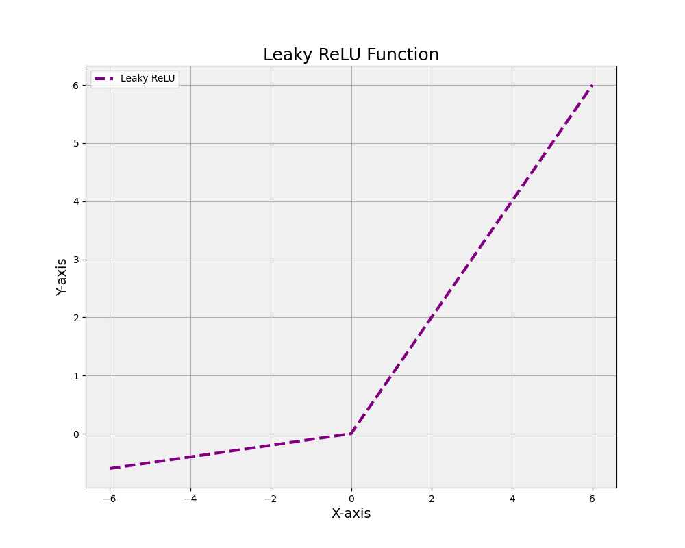
7. Leaky ReLU Neuron

A variation of the ReLU neuron, where the Leaky ReLU activation function allows a small, non-zero output for negative input values. This helps mitigate the “dying ReLU” problem, where some ReLU neurons become inactive during training and no longer contribute to learning.

8. Tanh Neuron

A neuron with a hyperbolic tangent (tanh) activation function, which maps the weighted sum of inputs to a value between -1 and 1. Tanh neurons are similar to sigmoid neurons, but with a broader output range and a stronger gradient for input values close to zero.

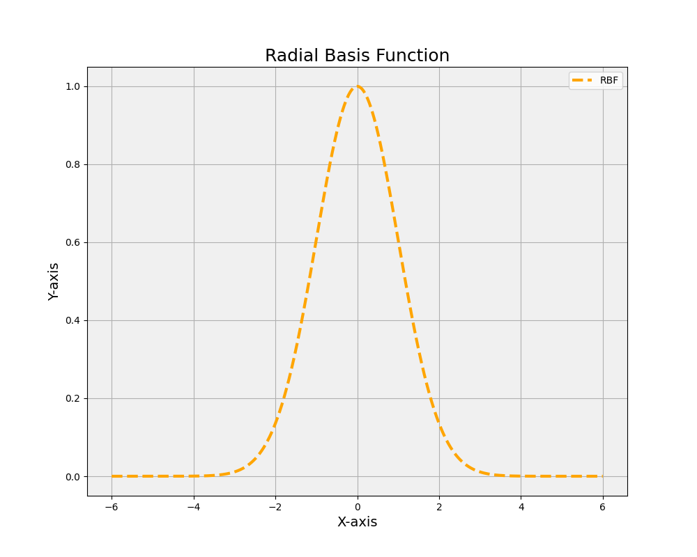
9. Radial Basis Function (RBF) Neuron

This neuron has a Gaussian-like activation function, which measures the similarity between its input and a reference point (center). RBF neurons are commonly used in RBF networks for tasks like function approximation and clustering.

10. Layer

A layer in the context of deep learning refers to a collection of artificial neurons organized within a neural network. Layers are the basic building blocks of a neural network architecture and can be categorized into three main types:

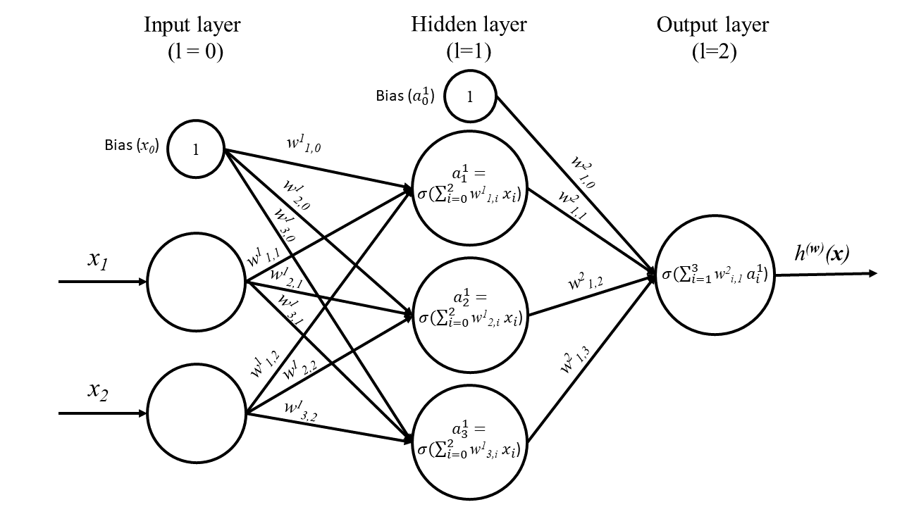
11. Input Layer

This is the first layer of a neural network that receives input data, such as raw features, images, or text. Each neuron in the input layer corresponds to a single feature or data point. The input layer does not perform any computation or transformation on the input data.

12. Hidden Layer(s)

These are the layers between the input and output layers, where the actual computation and learning occur. A neural network can have multiple hidden layers, and each layer may consist of a different number of neurons. The neurons in the hidden layers apply activation functions to the weighted sum of inputs from the previous layer, transforming and propagating the data through the network.

13. Output Layer

The final layer in a neural network, which produces the output or prediction. The number of neurons in the output layer depends on the task and desired output format. For example, in a binary classification problem, there might be one output neuron with a sigmoid activation function, while in a multi-class problem, there might be multiple neurons with a softmax activation function.

Layers can be fully connected (dense) or have other structures such as convolutional layers, recurrent layers, or attention layers, depending on the network architecture and the problem being addressed. In deep learning, networks often have multiple hidden layers, which allows them to learn complex, hierarchical representations of the input data, leading to better performance in tasks such as image recognition, natural language processing, and reinforcement learning.

14. Neural Network (NN) and Artificial Neural Network (ANN)

A neural network, also known as an artificial neural network (ANN), is a machine-learning model inspired by the structure and functioning of biological neural networks in the human brain. It consists of interconnected artificial neurons organized into layers, which process and transmit information through weights, biases, and activation functions. Neural networks are widely used in machine learning and deep learning for tasks such as pattern recognition, image and speech recognition, natural language processing, and reinforcement learning.

A neural network typically has three main types of layers, which are the input layer, hidden layer(s), and the output layer.

The learning process in a neural network involves adjusting the weights and biases through optimization algorithms, such as gradient descent, to minimize the error between the network’s predictions and the correct outputs. This process is typically carried out through a combination of forward and backward passes, where the network computes the output based on the input data and then updates the weights and biases based on the error.

Neural networks can have various architectures, such as feedforward networks, convolutional neural networks (CNNs), recurrent neural networks (RNNs), and transformers, each suited for different types of problems and data. The choice of architecture, activation functions, and optimization algorithms depends on the specific problem being addressed and the desired properties of the model.

15. Weights, 16. Biases, and 17. Connections

In a neural network, weights, biases, and connections play crucial roles in processing and learning from input data. Let’s look at each term in detail:

• Weights: Weights are numerical values associated with the connections between neurons in a neural network. Each connection between two neurons has a weight that represents the strength or influence of one neuron’s output on another neuron’s input. During the learning process, the neural network adjusts these weights to minimize the error between its predictions and the correct output, effectively learning the underlying patterns in the data. Weights can be positive (excitatory) or negative (inhibitory), which indicates whether the connection amplifies or dampens the signal, respectively.
• Biases: Biases are additional parameters in a neural network, acting as a constant term that is added to the weighted sum of inputs for each neuron. The bias allows the neuron to shift its activation function along the input axis, enabling the network to learn more complex decision boundaries and better fit the data. Like weights, biases are adjusted during the learning process to minimize the prediction error.
• Connections: Connections in a neural network are the links between neurons that transmit signals from one neuron to another. Each connection has an associated weight, and the signal passing through a connection is multiplied by its weight. In fully connected layers, each neuron is connected to every neuron in the adjacent layers, whereas in other layer types, such as convolutional or recurrent layers, the connections have specific patterns and structures.

For example, consider a simple feedforward neural network with an input layer, one hidden layer, and an output layer. The input layer neurons are connected to the hidden layer neurons with connections that are associated with weights, and the hidden layer neurons are connected to the output layer neurons through another set of connections associated with weights. During the forward pass, the network computes the weighted sum of inputs for each neuron in the hidden layer, adds the bias, and applies an activation function. The same process is repeated for the output layer neurons to produce the final prediction. During the backward pass, the network adjusts the weights and biases based on the error between the prediction and the correct output, using optimization algorithms such as gradient descent.

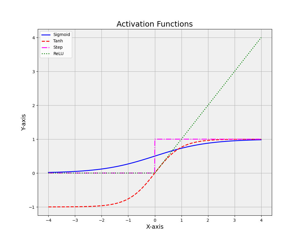
18. Activation Function (also known as Transfer Function)

An activation function, also known as a transfer function, plays a crucial role in artificial neural networks. The primary purpose of an activation function is to introduce non-linearity into the neural network, enabling it to learn complex, non-linear relationships between input features and output predictions.

In a neural network, individual neurons receive input signals from connected neurons in the previous layer. The activation function processes these inputs, transforming them into a single output value. This output then serves as an input to neurons in the next layer. By applying a non-linear transformation, the activation function allows the neural network to model complex, non-linear patterns in the data, which would be challenging or impossible for linear models.

There are several commonly used activation functions in machine learning, each with its strengths and weaknesses. Some popular examples include:

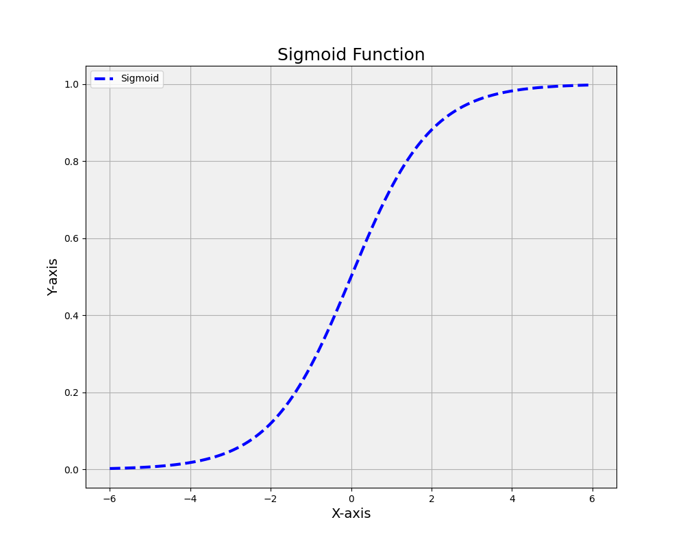
19. Sigmoid function (also known as the logistic function)

This S-shaped function maps input values to the range (0, 1), making it suitable for binary classification tasks or when interpreting output as probabilities. However, it can suffer from the vanishing gradient problem, where the gradients become very small during training, causing slow learning.

The sigmoid function is mathematically defined as:

σ(x) = 1 / (1 + e^-x)

Where:

• σ(x) is the output of the sigmoid function for a given input x.
• e is the base of the natural logarithm (approximately equal to 2.71828).
• x is the input to the function.

This function maps any input x to a value between 0 and 1. It’s commonly used in machine learning and artificial intelligence, particularly in logistic regression and neural networks, due to its useful properties for those applications, such as having a well-defined derivative.

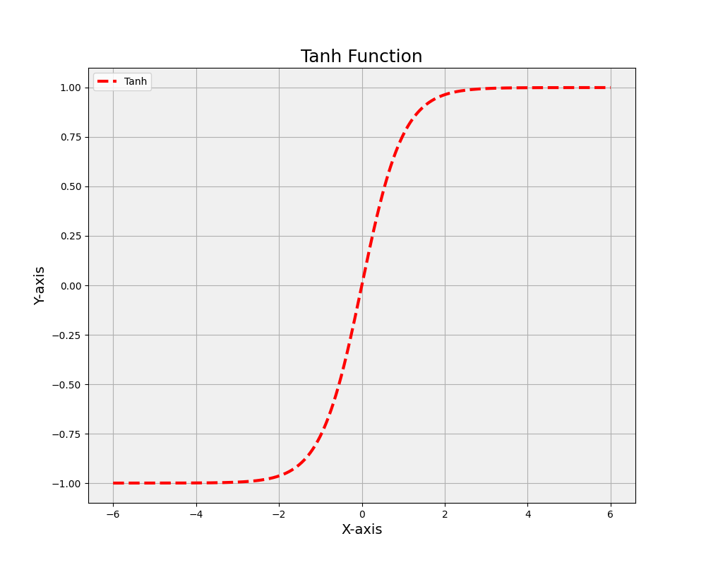
20. Hyperbolic tangent (tanh) function

Similar to the sigmoid function, the tanh function has an S-shape but maps input values to the range (-1, 1). This centered output can lead to faster convergence during training, but it also shares the vanishing gradient problem with the sigmoid function

The hyperbolic tangent function is defined mathematically as:

tanh(x) = (e^x – e^-x) / (e^x + e^-x)

Where:

• tanh(x) is the output of the tanh function for a given input x.
• e is the base of the natural logarithm (approximately equal to 2.71828).
• x is the input to the function.

This function maps any real-valued number to the range -1 to 1. It’s also frequently used in machine learning and artificial intelligence, especially in neural networks, as an activation function. Compared to the sigmoid function, the tanh function is zero-centered, making it often easier to model inputs that have strongly negative, neutral, or strongly positive values.

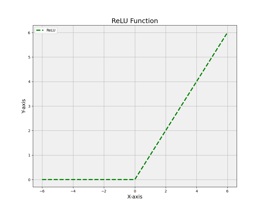
21. Rectified Linear Unit (ReLU) function

The ReLU function outputs the input value if it is positive and zero otherwise. It has become a popular choice due to its computational efficiency and ability to mitigate the vanishing gradient problem. However, ReLU units can suffer from the “dying ReLU” issue, where some neurons become inactive and stop learning.

The ReLU function is mathematically defined as:

ReLU(x) = max(0, x)

Where:

• ReLU(x) is the output of the ReLU function for a given input x.
• x is the input to the function.

This function will output the input directly if it’s positive; otherwise, it will output zero. This means that it effectively “rectifies” negative inputs to zero. It has been found to work well in practice for many types of neural networks, partly because its simplicity helps to mitigate the vanishing gradient problem that can occur with other activation functions.

22. Leaky ReLU

The Leaky Rectified Linear Unit (Leaky ReLU) is a variation of the standard ReLU activation function, designed to address the “dying ReLU” problem, where neurons with negative inputs become inactive and stop learning. Leaky ReLU introduces a small positive slope for negative inputs, allowing a tiny gradient to flow through the neuron and maintaining its ability to learn. The mathematical formula for Leaky ReLU is f(x) = max(αx, x), where x is the input, α is a small positive constant (typically around 0.01), and f(x) is the output. By allowing a non-zero gradient for negative inputs, Leaky ReLU mitigates the dying ReLU issue and can improve the stability of the training process.

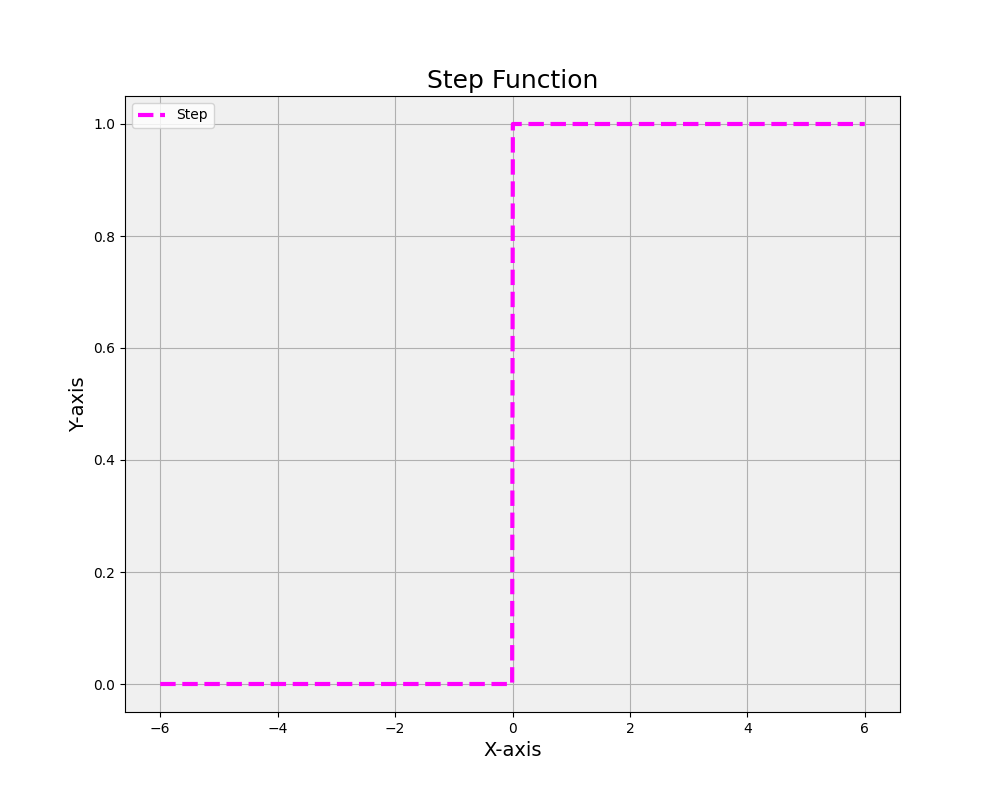
23. Step function

The step function is a binary activation function that produces an output of 1 if the input is greater than or equal to a predefined threshold, and 0 otherwise. Mathematically, it is expressed as f(x) = 1 if x >= θ, and f(x) = 0 if x < θ, where x is the input, θ is the threshold, and f(x) is the output. The step function is simple and easy to compute; however, it is non-differentiable and discontinuous, making it unsuitable for gradient-based optimization methods that utilize backpropagation, used in deep learning. As a result, the step function is generally not used in modern neural networks, and smoother, differentiable activation functions like sigmoid, tanh, or ReLU are preferred.

24. Radial Basis Function (RBF)

The Radial Basis Function is an activation function primarily used in Radial Basis Function Networks (RBFNs), a type of artificial neural network. RBF is a real-valued function that depends on the distance between the input and a center point, usually in the form of a Gaussian function. The most common RBF is the Gaussian function, defined as f(x) = exp(-||x – c||^2 / (2σ^2)), where x is the input, c is the center point, σ is the width parameter, and f(x) is the output. The RBF activation function is highly sensitive to the proximity of the input to the center point, making it suitable for tasks like function approximation, interpolation, and pattern recognition. However, RBF is less common in deep learning, where ReLU and its variants are more widely used.

In summary, an activation function, or transfer function, is a critical component in neural networks that introduces non-linearity, allowing the network to learn complex relationships in the data. Different activation functions, such as sigmoid, tanh, and ReLU, have unique properties that make them more suitable for specific tasks or network architectures. Choosing the right transfer function can significantly impact the performance and efficiency of a neural network in machine learning applications.

25. Forward Propagation, Forward Pass, or Inference

Forward propagation, also known as the forward pass or inference, is the process of computing the output of a neural network given its input data and the current values of weights and biases. During forward propagation, information flows from the input layer through the hidden layers to the output layer, with each neuron applying an activation function to the weighted sum of its inputs and biases. This process generates the network’s prediction or output for the given input data.

26. Backpropagation

Backpropagation, short for “backward propagation of errors,” is a widely used efficient algorithm for computing the gradient of the loss function, which is required by most optimization algorithms in supervised learning for training artificial neural networks. It is a form of supervised learning because it requires labeled data to compute the error between the network’s predictions and the correct outputs. The backpropagation algorithm calculates the gradient of the loss function in terms of each weight and bias by applying the chain rule, computing the gradient one layer at a time, iterating backward from the last layer to the first.

Here’s a detailed step-by-step explanation of how the backpropagation algorithm is used:

1. Initialization: Initialize the neural network with random weights and biases.
2. Forward Pass: Given an input sample and the current weights and biases, compute the output of the network layer by layer, starting from the input layer, passing through the hidden layers, and reaching the output layer. For each neuron, compute the weighted sum of inputs, add the bias, and apply the activation function.
3. Compute Loss: Calculate the loss (error) between the network’s output and the correct output (label) using a predefined loss function, such as mean squared error (MSE) for regression or cross-entropy loss for classification.
4. Backward Pass: Compute the gradient of the loss function with respect to each weight and bias in the network by applying the chain rule, iterating backward from the output layer to the input layer.
   • Output Layer: Calculate the gradient of the loss with respect to the output layer’s activations (sometimes denoted as ‘delta’), which depends on the chosen loss function and the activation function used in the output layer.
   • Hidden Layers: For each hidden layer, starting from the last hidden layer and moving toward the input layer, compute the gradient of the loss with respect to the activations of that layer. This involves multiplying the gradient from the previous (higher) layer by the derivative of the activation function and the weights connecting the layers.
   • Weights and Biases: Compute the gradient of the loss with respect to each weight and bias in the network. This is done by multiplying the gradient of the loss with respect to the activations (calculated in steps 4a and 4b) by the corresponding input or activation values for weights and a constant 1 for biases.
5. Update Weights and Biases: Update the weights and biases using the computed gradients and a predefined learning rate. This is typically done using the gradient descent algorithm or one of its variants, such as stochastic gradient descent (SGD), Adam, or RMSprop.
6. Repeat: Perform steps 2-5 for a predefined number of epochs or until a convergence criterion is met, such as a minimum change in the loss function or reaching a maximum number of iterations.

The backpropagation algorithm allows neural networks to learn complex, non-linear relationships between inputs and outputs by iteratively adjusting the weights and biases to minimize the prediction error. It is a computationally efficient method for training deep neural networks and forms the basis for many modern deep learning techniques.

27. Feedforward network

A feedforward network, also known as a feedforward neural network, is a type of artificial neural network where the connections between neurons do not form any cycles or loops. Information in a feedforward network flows in one direction, starting from the input layer, passing through any hidden layers, and ending at the output layer. This unidirectional flow of information differentiates feedforward networks from recurrent neural networks (RNNs), which have connections that loop back and can maintain hidden states across time steps.

The architecture of a feedforward network typically consists of an input layer, one or more hidden layers, and an output layer. Each layer consists of a set of artificial neurons that apply activation functions to the weighted sum of inputs from the previous layer (plus the bias).

Feedforward networks are widely used for a variety of machine learning tasks, such as classification, regression, and pattern recognition. They are trained using supervised learning techniques and optimization algorithms like gradient descent, which adjusts the weights and biases of the network to minimize the error between the network’s predictions and the correct outputs.

Some common types of feedforward networks include:

• Multi-Layer Perceptron (MLP): A fully connected feedforward network with one or more hidden layers. MLPs can learn complex, non-linear relationships between inputs and outputs.
• Convolutional Neural Network (CNN): A specialized feedforward network designed for processing grid-like data, such as images. CNNs consist of convolutional layers, pooling layers, and fully connected layers to learn hierarchical features and perform tasks like image classification and object detection.
• Radial Basis Function Network (RBFN): A feedforward network that uses radial basis functions as activation functions in the hidden layer, making it particularly suited for tasks like function approximation and interpolation.

While feedforward networks are powerful and versatile, their lack of internal state and cyclical connections limits their ability to handle sequential data and capture temporal dependencies, which is where recurrent neural networks (RNNs) and other sequence-processing architectures excel.

28. Multilayer Perceptron (MLP) and Regular Neural Network (RNN)

A multilayer perceptron (MLP), sometimes also called a regular neural network (RNN) (not to be confused with a recurrent neural network, also RNN for short), is a type of feedforward artificial neural network that consists of an input layer, one or more hidden layers, and an output layer. MLPs are characterized by their fully connected architecture, where each neuron in a layer is connected to every neuron in the adjacent layers. MLPs can learn complex, non-linear relationships between inputs and outputs, making them suitable for a wide range of machine learning tasks, such as classification and regression.

An MLP is trained using supervised learning techniques, with gradient descent and its variants being the most common algorithms for adjusting weights and biases to minimize the error between the network’s predictions and the correct outputs. Activation functions, such as sigmoid, ReLU, or tanh, are applied to the weighted sums of inputs and biases to introduce non-linearity in the network.

29. Fully Connected Layer (also known as Dense layer)

A fully connected (or dense) layer is a type of layer in a neural network where each neuron in the layer is connected to every neuron in the previous and following layers. In the context of an MLP, all hidden layers and the output layer are fully connected layers. The neurons in a fully connected layer compute the weighted sum of their inputs from the previous layer, add a bias term, and apply an activation function to produce an output that is passed to the next layer. Fully connected layers enable the network to learn high-level abstractions and complex relationships between inputs and outputs, making them a crucial component of many neural network architectures.

30. Autoencoder

An autoencoder is a type of artificial neural network used for unsupervised learning tasks, particularly for dimensionality reduction and feature learning. Autoencoders are designed to learn a compressed representation of input data by reconstructing the input as accurately as possible, effectively forcing the network to capture the most important features and patterns in the data.

An autoencoder consists of two main components:

1. Encoder: The encoder is a neural network that maps the input data to a lower-dimensional latent space, effectively compressing the data. The encoder learns to extract meaningful features from the input and represents them in a compact form. The output of the encoder is called the “code” or “latent representation.”
2. Decoder: The decoder is another neural network that maps the latent representation back to the original input space, attempting to reconstruct the input data. The decoder learns to recreate the original input data from the compressed representation provided by the encoder.

During training, autoencoders minimize the reconstruction error between the original input data and the reconstructed data produced by the decoder. This process encourages the encoder to learn a compressed representation that retains the most important information while discarding any noise or irrelevant details.

Autoencoders have been used in various applications, such as:

• Dimensionality reduction: Autoencoders can be used as a non-linear alternative to techniques like PCA, learning more expressive low-dimensional representations of the input data.
• Feature learning: The latent representation learned by the encoder can be used as a set of high-level features for other machine learning tasks, such as classification or clustering.
• Denoising: Autoencoders can be trained to reconstruct clean input data from noisy input samples, effectively learning to denoise the data.
• Anomaly detection: Autoencoders can be used to detect anomalous or unusual data points by measuring the reconstruction error, as they tend to have higher errors when reconstructing samples that deviate from the normal data distribution.

Variants of autoencoders, such as variational autoencoders (VAEs) and denoising autoencoders, have been developed to address specific tasks or improve the learning capabilities of the basic autoencoder architecture.

31. Convolutional Neural Network (CNN)

A Convolutional Neural Network (CNN) is a type of deep learning model and an artificial neural network particularly well-suited for processing grid-like data, such as images or speech signals. CNNs achieve this by employing convolutional layers, which are specifically designed to capture local patterns and spatial relationships in the input data. These layers work in conjunction with other types of layers, such as fully connected layers, to learn hierarchical representations and make predictions.

32. Convolution

A convolution, in the context of machine learning, is a mathematical operation that involves sliding a small matrix called the kernel or filter over the input data. For each position of the kernel, a local region in the input data is multiplied element-wise with the kernel, and the results are summed up to produce a single value in the output. This process is repeated across the entire input data, generating a new matrix called the feature map. The convolution operation helps identify and extract features from the input data, like edges, corners, or textures in the case of images.

33. Convolutional Layer

A convolutional layer is a core component of a CNN, responsible for performing the convolution operation on the input data or on the output from previous layers. Each convolutional layer consists of multiple filters, with each filter designed to detect a specific feature in the input data. As the input passes through multiple convolutional layers in a CNN, the network progressively learns to recognize more complex and abstract patterns. The depth of the layer, or the number of filters, determines the number of feature maps generated in that layer. These feature maps are then passed on to subsequent layers, allowing the network to build a hierarchical understanding of the input data.

In summary, a Convolutional Neural Network is a type of deep learning model that uses convolutional layers to process grid-like data. These layers perform convolutions on the input data, generating feature maps that capture local patterns and spatial relationships. The convolutional layers work together with other layer types in a CNN to learn hierarchical representations and make predictions.

34. Pooling, 35. Average Pooling, and 36. Max Pooling

Pooling is an operation used in Convolutional Neural Networks to reduce the spatial dimensions of feature maps, which helps decrease computational complexity and control overfitting. By performing pooling, the network becomes more robust to small spatial variations in the input data and focuses on the most important features. Pooling is typically applied after one or more convolutional layers and can be performed using different methods, such as Average Pooling and Max Pooling.

Average Pooling is a type of pooling operation that calculates the average value of a local region in the feature map. To perform average pooling, a small window or filter is slid over the input data in a similar manner to convolution. For each position of the window, the average value of the pixels within that region is computed and used as the output value in the corresponding location of the pooled feature map. This process is repeated for the entire feature map, resulting in a smaller, downsampled version that retains the general spatial structure of the input data while reducing its dimensions.

Max Pooling is another common pooling method that selects the maximum value from a local region in the feature map. Like average pooling, max pooling involves sliding a small window over the input data. However, instead of computing the average value, max pooling selects the highest value within the local region for each position of the window. This operation effectively captures the most prominent features in the input data while discarding less important details. Max pooling is particularly useful for detecting the presence of specific features, regardless of their exact location within the region.

37. Activation Map

An activation map is a two-dimensional grid that represents the output of a specific filter or convolution in a convolutional neural network. The filters in a CNN are small matrices of weights that are applied to specific regions of an input image to extract relevant features, such as edges or corners. Each filter produces a single output known as a feature map, and the collection of all feature maps produced by a layer of filters is known as the activation map.

The activation map provides information on the activation levels of the features detected by a particular filter in the CNN. High activation levels indicate that the feature is present in the input image, while low activation levels suggest that the feature is not present. The activation map is a useful tool for visualizing and interpreting the output of a CNN, as it can help to identify the specific features that are most relevant for a given image recognition task.

38. Convolutional Autoencoder

A Convolutional Autoencoder is a type of unsupervised deep learning model that leverages the structure of Convolutional Neural Networks to learn useful representations of input data, typically images, without the need for labeled data. An autoencoder consists of two main components: an encoder, which compresses the input data into a lower-dimensional representation or code, and a decoder, which reconstructs the original input data from this lower-dimensional representation. Convolutional Autoencoders utilize convolutional layers in both the encoder and decoder parts, enabling them to capture spatial patterns and hierarchies more effectively than traditional autoencoders that use fully connected layers.

In the encoding phase, a Convolutional Autoencoder processes the input data through a series of convolutional layers, typically followed by pooling layers to reduce the spatial dimensions. These layers work together to capture increasingly complex features and patterns in the input data, while compressing it into a more compact representation. The encoder essentially learns to identify the most important information in the input data and discards less relevant details.

The decoding phase of a Convolutional Autoencoder aims to reconstruct the original input data from the compressed representation generated by the encoder. The decoder uses a series of upsampling and convolutional layers to achieve this goal. Upsampling layers increase the spatial dimensions of the data, while convolutional layers help refine the reconstruction and ensure that the output resembles the original input as closely as possible. The decoder learns to reverse the transformations applied by the encoder, effectively generating a high-quality approximation of the original input data.

Convolutional Autoencoders have various applications, including image denoising, feature extraction, and unsupervised learning of representations for downstream tasks. By training the model to minimize the reconstruction error between the input and the output, a Convolutional Autoencoder can learn meaningful and robust representations of the data that can be used for tasks such as classification or clustering when labeled data is scarce or unavailable.

39. Recurrent Neural Network (RNN)

A recurrent neural network (RNN) is a type of artificial neural network specifically designed to handle sequential data and capture temporal dependencies. RNNs are characterized by their ability to maintain an internal hidden state that can store information from previous time steps, allowing them to process input sequences of varying lengths and learn patterns across time.

In an RNN, connections between neurons form directed cycles, enabling the network to maintain a hidden state that can be updated at each time step as new inputs are received. This contrasts with feedforward neural networks, where information flows only in one direction from input to output, without any cycles or loops.

RNNs are particularly useful for tasks that involve time series data, natural language processing, speech recognition, and other problems where the order of the input data is important. The ability to capture temporal dependencies makes RNNs a powerful tool for modeling sequences and learning patterns over time.

However, traditional RNNs can struggle to learn long-range dependencies due to issues like vanishing and exploding gradients during training. To address these challenges, more advanced RNN architectures, such as Long Short-Term Memory (LSTM) and Gated Recurrent Units (GRU), have been developed. These architectures incorporate gating mechanisms that allow them to better capture long-range dependencies and improve learning performance in various tasks.

40. Hidden state

The hidden state in a recurrent neural network (RNN) is an internal representation of the information captured from previous time steps in a sequence. It serves as a form of memory, allowing the RNN to maintain context and learn patterns across time steps in the input data.

At each time step, an RNN computes its hidden state based on the input at the current time step and the hidden state from the previous time step. The hidden state is then used to compute the output of the RNN at the current time step and passed on to the next time step to maintain context.

In RNN variants like Long Short-Term Memory (LSTM) networks and Gated Recurrent Units (GRU), the hidden state works in conjunction with gating mechanisms and, in the case of LSTMs, an additional cell state. These mechanisms help the network selectively retain or forget information from previous time steps, making them more effective at capturing long-range dependencies in the input data.

41. Backpropagation Through Time (BPTT)

Backpropagation Through Time (BPTT) is an extension of the backpropagation algorithm specifically designed for training recurrent neural networks. BPTT works by unrolling the RNN over a fixed number of time steps and applying the standard backpropagation algorithm to the resulting unfolded network.

Here’s a high-level overview of the BPTT algorithm:

1. Unroll the RNN: Given a sequence of input data, unroll the RNN for a fixed number of time steps (T), creating a feedforward-like network where each layer corresponds to a specific time step.
2. Forward Pass: Perform forward propagation through the unrolled network, computing the hidden states and outputs for each time step.
3. Compute Loss: Calculate the loss between the network’s output and the correct output (label) for each time step. The total loss is the sum of the individual time step losses.
4. Backward Pass: Apply the standard backpropagation algorithm to the unrolled network, computing the gradient of the loss function concerning each weight and bias at each time step.
5. Update Weights and Biases: Update the weights and biases using the computed gradients and a predefined learning rate, typically using the gradient descent algorithm or one of its variants.
6. Repeat: Perform steps 2-5 for a predefined number of epochs or until a convergence criterion is met.

BPTT allows RNNs to learn complex, temporal relationships between inputs and outputs by iteratively adjusting the weights and biases to minimize the prediction error across time steps. However, BPTT can suffer from issues like vanishing and exploding gradients when dealing with long sequences, leading to difficulties in learning long-range dependencies. To address these issues, more advanced RNN architectures like Long Short-Term Memory (LSTM) and Gated Recurrent Units (GRU) have been developed.

42. Long Short-Term Memory (LSTM)

Long Short-Term Memory (LSTM) is a type of recurrent neural network (RNN) architecture designed to address the vanishing gradient problem often encountered in training traditional RNNs. LSTMs are particularly effective at capturing long-range dependencies in sequential data, making them suitable for various tasks involving time series, natural language processing, speech recognition, and more.

LSTM networks introduce a unique gating mechanism that enables them to selectively retain or forget information across time steps. This mechanism consists of three gates: the input gate, the forget gate, and the output gate. Additionally, LSTMs maintain a cell state, which serves as an internal memory for the network.

1. Input gate: The input gate determines how much of the new input at the current time step should be incorporated into the cell state. It uses a sigmoid activation function to produce values between 0 and 1, where 0 means ignoring the input completely, and 1 means accepting the entire input.
2. Forget gate: The forget gate decides how much of the previous cell state should be retained or forgotten at the current time step. Similar to the input gate, the forget gate uses a sigmoid activation function to produce values between 0 and 1, where 0 means forgetting the entire cell state, and 1 means retaining it completely.
3. Output gate: The output gate determines how much of the updated cell state should be used to produce the output of the LSTM unit at the current time step. The output gate also uses a sigmoid activation function to produce values between 0 and 1, controlling the amount of cell state information passed to the output.

The LSTM’s gating mechanism and cell state allow it to effectively learn and maintain long-range dependencies in the input data, overcoming the limitations of traditional RNNs. LSTMs have been widely adopted in various applications, such as machine translation, text generation, speech recognition, and video analysis, among others.

43. Gated Recurrent Units (GRU)

Gated Recurrent Units (GRU) are a type of recurrent neural network (RNN) architecture designed to capture long-range dependencies in sequential data more effectively than traditional RNNs, while being computationally more efficient than Long Short-Term Memory (LSTM) networks. GRUs were introduced by Kyunghyun Cho et al. in 2014 and have been successfully applied to various tasks, including natural language processing, speech recognition, and time series analysis.

GRUs employ a gating mechanism similar to LSTMs but with a simpler structure. They feature two gates: the update gate and the reset gate.

1. Update gate: The update gate is responsible for determining the degree to which the previous hidden state should be maintained or updated with new information at the current time step. The update gate uses a sigmoid activation function, producing values between 0 and 1, where 0 means replacing the hidden state entirely with new information, and 1 means retaining the entire previous hidden state.
2. Reset gate: The reset gate controls how much of the previous hidden state should be used to compute the candidate hidden state, which is a proposed update for the current hidden state. The reset gate also uses a sigmoid activation function to produce values between 0 and 1, where 0 means ignoring the previous hidden state completely, and 1 means considering the entire previous hidden state.

GRUs simplify the LSTM architecture by combining the input and forget gates into a single update gate and using the same hidden state as the memory cell. This reduces the number of parameters in the model, making GRUs faster to train and less memory-intensive than LSTMs, while still being capable of modeling long-range dependencies.

In practice, the choice between LSTMs and GRUs depends on the specific problem and the available computational resources. In some cases, GRUs may perform comparably to LSTMs with fewer parameters and faster training times, while in other cases, LSTMs may provide better performance at the cost of increased complexity.

44. Generative models

Generative models are a class of machine learning models that aim to learn the underlying probability distribution of the training data and generate new samples that resemble the original data. They capture the structure, patterns, and variations in the data, allowing them to create synthetic instances that share similar properties with the real-world examples.

Generative models have a wide range of applications, including image synthesis, text generation, speech synthesis, drug discovery, and data augmentation, among others. There are several types of generative models, some of the most popular ones include:

• Generative Adversarial Networks (GANs): GANs consist of two neural networks, a generator and a discriminator, that compete against each other in a zero-sum game. The generator learns to create realistic samples, while the discriminator learns to distinguish between real and generated samples. The process continues iteratively until the generator produces samples that the discriminator can no longer distinguish from real data.
• Variational Autoencoders (VAEs): VAEs are a type of autoencoder that learns a probabilistic mapping between the input data and a lower-dimensional latent space. VAEs impose a specific structure on the latent space, usually by constraining it to follow a Gaussian distribution, which encourages the model to learn a smooth and continuous representation of the data. New samples can be generated by decoding points sampled from the latent space.
• Restricted Boltzmann Machines (RBMs): RBMs are a type of shallow generative model that consists of two layers, a visible layer representing the input data and a hidden layer representing latent features. The model learns a joint probability distribution over the visible and hidden layers, and new samples can be generated by sampling from this distribution.
• Bayesian Networks: Bayesian networks are probabilistic graphical models that represent the dependencies among a set of random variables using a directed acyclic graph. They can be used to model the joint probability distribution of the variables and generate new samples by sampling from the learned distribution.

Generative models are powerful tools for learning complex data distributions and generating new data samples, but they can be challenging to train and may require large amounts of data and computational resources to achieve high-quality results.

45. Sequence-to-sequence (seq2seq) models

Sequence-to-sequence (seq2seq) models are a class of deep learning models designed to map an input sequence to an output sequence, where the lengths of the input and output sequences may differ. Seq2seq models are widely used in natural language processing tasks, such as machine translation, text summarization, and speech recognition, as well as other domains like time-series prediction and video captioning.

A typical seq2seq model consists of two main components:

1. Encoder: The encoder processes the input sequence and encodes its information into a fixed-size latent representation, often called the context vector or hidden state. The encoder can be built using various neural network architectures, such as recurrent neural networks (RNNs), long short-term memory networks (LSTMs), or Transformers.
2. Decoder: The decoder takes the context vector generated by the encoder and generates the output sequence, one element at a time. Like the encoder, the decoder can be constructed using RNNs, LSTMs, or Transformers. During the generation process, the decoder typically utilizes techniques such as teacher forcing, scheduled sampling, or beam search to improve the quality and efficiency of the output sequence.

Seq2seq models can be trained using supervised learning, where pairs of input-output sequences are used to adjust the model’s parameters. The training objective is often to minimize the cross-entropy loss between the model’s predicted output sequence and the ground-truth output sequence.

Although seq2seq models have been successful in various applications, they face challenges like handling long sequences and capturing long-range dependencies. Attention mechanisms, which allow the model to focus on relevant parts of the input sequence while decoding, have been introduced to address these challenges and have significantly improved seq2seq model performance across a range of tasks.

46. Transfer Learning

Transfer learning is a machine learning technique where a pre-trained model, typically developed for one task, is fine-tuned or adapted for a different but related task. This approach leverages the knowledge gained from the original task to improve the performance and reduce the training time for the new task. Transfer learning is particularly useful when dealing with limited labeled data for the target task, as it can make use of the more abundant data available for the original task.

Transfer learning is commonly used in deep learning, particularly with convolutional neural networks for image classification and natural language processing models like BERT or GPT. The idea is that the pre-trained model has already learned useful features or representations from the original task, which can be beneficial for the target task. In the context of CNNs, the lower layers of the network typically learn general features like edges and textures, while the higher layers learn more task-specific features.

There are two main approaches to transfer learning:

1. Feature extraction: In this approach, the pre-trained model is used as a fixed feature extractor, and the output from one of its layers is fed into a new classifier, which is trained for the target task. The weights of the pre-trained model are not updated during training for the new task. This approach is suitable when the target task’s dataset is small, and fine-tuning the entire network might lead to overfitting.
2. Fine-tuning: In this approach, the pre-trained model is used as a starting point, and its weights are updated during training for the target task. Often, only a subset of the layers, such as the higher layers, is fine-tuned, while the lower layers are kept fixed. Fine-tuning is typically done with a smaller learning rate to preserve the previously learned features while adapting the model to the new task.

Transfer learning has become a widely used technique in deep learning, as it can significantly improve the model’s performance and reduce the computational resources required for training, especially when dealing with limited labeled data for the target task.

47. Generative Adversarial Network (GAN)

Generative Adversarial Networks (GANs) are a class of deep learning models that can generate new data samples resembling the original data. GANs consist of two neural networks, a Generator and a Discriminator, that compete against each other in a zero-sum game. The Generator learns to create realistic synthetic data, while the Discriminator learns to distinguish between real and generated samples.

How GANs work:

1. The Generator takes a random noise vector as input and generates a synthetic data sample.
2. The Discriminator receives both real data samples and the generated samples from the Generator.
3. The Discriminator’s objective is to correctly classify samples as real or generated. It is trained to minimize the classification error.
4. The Generator’s objective is to create samples that are indistinguishable from real data. It is trained to maximize the classification error of the Discriminator.
5. The training process involves alternating between training the Discriminator and the Generator, in a process akin to a game of cat and mouse.

Why GANs are important:

GANs can generate high-quality samples, making them useful in various applications such as image synthesis, data augmentation, and style transfer. For example, GANs can create realistic images of faces that do not exist, generate artwork in the style of a particular artist, or even enhance low-resolution images.

48. Zero-sum game

A zero-sum game is a situation in game theory where the total gain or loss among all players is always zero. In other words, one player’s gain comes at the expense of another player’s loss. The concept is based on the idea that the total amount of resources in a system is fixed, and players compete for shares of these resources.

In the context of GANs, the zero-sum game is a metaphor for the adversarial relationship between the Generator and Discriminator. The Generator tries to create realistic samples, while the Discriminator tries to identify whether a sample is real or generated. As the Generator becomes better at producing realistic samples, the Discriminator’s ability to correctly classify them decreases. Conversely, as the Discriminator becomes better at classifying samples, the Generator is forced to improve its sample generation. This dynamic pushes both networks to improve continuously, ultimately leading to the generation of high-quality synthetic data.

49. Attention and Attention Mechanism

The phrase “Attention is all you need” refers to a landmark paper published in 2017 by Vaswani et al., which introduced the Transformer architecture. The paper’s title, “Attention Is All You Need,” highlights the authors’ claim that attention mechanisms are sufficient for solving complex tasks like machine translation, without the need for traditional recurrent neural networks or convolutional neural networks.

Attention is a concept in deep learning that allows models to selectively focus on specific parts of the input data when processing it. The attention mechanism helps models to weigh the importance of different input elements and allocate more computational resources to the most relevant ones. This concept is particularly useful in tasks like machine translation, where understanding the relationships between words in a sentence is crucial.

The attention mechanism works by computing a set of attention scores for each input element, which determines the amount of focus the model should allocate to that element. These scores are then used to create a weighted sum of input features, allowing the model to process the most relevant information in the context of the task at hand.

The Transformer architecture, which relies heavily on attention mechanisms, has become the foundation for many state-of-the-art models in natural language processing (NLP), such as BERT and GPT, due to its ability to effectively model long-range dependencies and parallelize computation for faster training.

Check out the explanation for the Transformer model below to learn more about Attention.

50. Transformer model

The Transformer is a deep learning model introduced by Vaswani et al. in the paper “Attention is All You Need.” It is primarily used for sequence-to-sequence tasks like machine translation and has become the foundation for many state-of-the-art models in natural language processing (NLP). The key innovation in the Transformer is its focus on self-attention mechanisms instead of traditional recurrent neural networks or convolutional neural networks.

High-level structure:

The Transformer model consists of an encoder and a decoder, both built from multiple layers of identical sub-modules.

1. Encoder: The encoder processes the input sequence and generates a continuous representation of the data. It consists of multiple identical layers, each with two main components: a Multi-Head Self-Attention mechanism and a Position-wise Feed-Forward Network.
2. Decoder: The decoder generates the output sequence from the encoded representation. Like the encoder, it has multiple identical layers, with three main components: a Multi-Head Self-Attention mechanism, a Multi-Head Encoder-Decoder Attention mechanism, and a Position-wise Feed-Forward Network.

Attention Mechanism:

The attention mechanism is the core component of the Transformer model. It allows the model to weigh the importance of different input elements and focus on the most relevant ones. The primary attention mechanism used in the Transformer is called Scaled Dot-Product Attention. It computes attention scores using the dot product of a query vector with key vectors, scaling the result, and applying a softmax function to obtain probabilities. The attention scores are then used to create a weighted sum of value vectors.

Multi-Head Attention:

To enhance the model’s ability to capture different types of relationships in the data, the Transformer employs Multi-Head Attention. This mechanism splits the input data into multiple parts or “heads,” allowing each head to focus on different aspects of the input. The results from each head are then concatenated and linearly transformed to produce the final output.

Position-wise Feed-Forward Networks:

These networks consist of two fully connected layers with a ReLU activation function between them. They are applied to each position separately and identically, allowing the model to learn non-linear interactions between input elements.

Positional Encoding:

Since the Transformer doesn’t have inherent knowledge of the input sequence’s position, it uses positional encoding to inject information about the position of each element in the sequence. Positional encodings are added to the input embeddings before being fed into the encoder and decoder. The authors of “Attention is All You Need” used sinusoidal functions with different frequencies as positional encodings, enabling the model to generalize to sequences of different lengths.

Training and Decoding:

The Transformer is trained using a standard cross-entropy loss function, with teacher forcing for the decoder. During decoding, it employs a technique called “beam search” to find the most likely output sequence.

In summary, the Transformer model, along with its attention mechanisms, has revolutionized NLP, enabling the development of highly effective models for various tasks, such as machine translation, text summarization, and sentiment analysis.

51. Teacher forcing

Teacher forcing is a training technique used in sequence-to-sequence models, such as the Transformer, or RNNs, where the model’s goal is to generate an output sequence based on an input sequence. Examples of such tasks include machine translation, text summarization, and image captioning.

In teacher forcing, during the training phase, the model’s ground-truth output from the previous time step is provided as input to the current time step instead of using the model’s own prediction. This approach helps the model to learn the correct sequence more efficiently, as it reduces the propagation of errors throughout the training process.

However, there is a discrepancy between the training and inference phases when using teacher forcing. During training, the model is exposed to the ground-truth sequence, while during inference, it generates the output based on its previous predictions. This discrepancy can lead to issues like exposure bias, where the model is not well-prepared to handle its own errors during inference.

To mitigate this issue, techniques like scheduled sampling or professor forcing have been proposed, which combine the benefits of teacher forcing with the model’s own predictions during training, making the training process more similar to the inference phase.

52. Professor forcing

Professor forcing is a technique designed to address the discrepancy between training and inference in sequence-to-sequence models, particularly when teacher forcing is employed. This discrepancy, known as exposure bias, arises because the model is exposed to ground-truth sequences during training, but it relies on its own predictions during inference.

Introduced by Alex Lamb et al. in the paper “Professor Forcing: A New Algorithm for Training Recurrent Networks,” professor forcing aims to make the training process more similar to the inference phase. The key idea is to train the model using two different behaviors: one that follows the ground-truth sequence (teacher forcing) and another that uses the model’s own predictions (free-running mode). These two behaviors are then aligned using a technique called adversarial training.

The training process in professor forcing involves three main components:

1. Encoder-Decoder Model: This is the primary sequence-to-sequence model being trained, with the encoder processing input sequences and the decoder generating output sequences.
2. Behavior Cloning: The model is first trained using teacher forcing to learn the ground-truth output sequence. This initial training helps the model learn the desired sequence without being influenced by its own errors.
3. Adversarial Training: An additional neural network called the Discriminator is introduced. The Discriminator’s goal is to distinguish between the hidden states generated by the model when using teacher forcing and when using its own predictions (free-running mode). The sequence-to-sequence model is then trained to minimize the Discriminator’s ability to differentiate between these two behaviors, effectively aligning them.

By aligning the model’s behavior in both teacher forcing and free-running modes, professor forcing mitigates the exposure bias issue, resulting in a model that is better prepared to handle its own errors during inference and potentially leading to improved performance in sequence generation tasks.

53. Scheduled sampling

Scheduled sampling is a technique used in training sequence-to-sequence models that aim to mitigate the exposure bias issue that arises when using teacher forcing. Exposure bias occurs due to the discrepancy between training and inference: during training, the model is exposed to ground-truth sequences, while during inference, the model relies on its own predictions. This discrepancy can result in poor performance when the model encounters its own errors during inference.

Proposed by Bengio et al. in the paper “Scheduled Sampling for Sequence Prediction with Recurrent Neural Networks,” scheduled sampling combines the benefits of teacher forcing with the model’s own predictions during the training process. The main idea is to gradually transition from using ground-truth sequences to using the model’s predictions as input for the next time step.

Scheduled sampling works as follows:

1. At the beginning of training, the model is trained using teacher forcing, where the ground-truth output from the previous time step is provided as input to the current time step.
2. As training progresses, the model is increasingly exposed to its own predictions. This is achieved by introducing a probability schedule, which determines the likelihood of using the model’s prediction instead of the ground-truth output for each time step.
3. The probability of using the model’s prediction starts low and gradually increases over time, following a predefined schedule (e.g., linear, exponential, or inverse sigmoid).
4. By the end of training, the model relies mostly on its own predictions, making the training process more similar to the inference phase.

Scheduled sampling helps the model learn to handle its own errors and be more robust during inference. However, it can sometimes introduce instability in training, as the model might be exposed to incorrect predictions early in the training process. Therefore, it is essential to choose an appropriate schedule for transitioning from teacher forcing to the model’s predictions to ensure stable learning.

54. Beam search

Beam search is a search algorithm used in sequence-to-sequence models during the decoding or inference phase to find the most likely output sequence. It is a heuristic approach that balances the trade-off between computational efficiency and the quality of the generated sequences. Beam search is particularly useful in tasks like machine translation, text summarization, and speech recognition.

The primary idea behind beam search is to maintain a fixed number of candidate partial sequences (called “beams”) at each time step, rather than exploring all possible sequences exhaustively. The algorithm works as follows:

1. At the first time step, the model generates a set of candidate tokens along with their probabilities.
2. The top K most probable tokens are selected, where K is the beam size. These tokens form the initial beams.
3. For each subsequent time step, the model extends each beam with all possible next tokens, creating K * |V| new candidates, where |V| is the size of the vocabulary.
4. The algorithm then selects the top K most probable sequences from these new candidates, and the process continues.
5. The search terminates when all beams reach the end-of-sequence token or a predefined maximum sequence length.
6. The beam with the highest overall probability is chosen as the final output sequence.

Beam search strikes a balance between greedy search, which selects the most probable token at each time step but may miss globally optimal sequences, and exhaustive search, which considers all possible sequences but is computationally infeasible. By adjusting the beam size, one can control the trade-off between search quality and computational complexity: larger beam sizes result in higher quality sequences but are more computationally expensive, while smaller beam sizes are faster but may produce suboptimal sequences.

55. Large language model (LLM)

Large Language Models (LLMs) are deep learning models designed to process and generate human-like natural language. These models are trained on vast amounts of text data and have a high capacity, allowing them to learn complex language patterns, structures, and even some factual knowledge. LLMs are primarily based on the Transformer architecture and its variants, which heavily utilize attention mechanisms.

Examples of LLMs include OpenAI’s GPT-3 (Generative Pre-trained Transformer 3), Google’s BERT (Bidirectional Encoder Representations from Transformers), and T5 (Text-to-Text Transfer Transformer). These models have achieved state-of-the-art performance across a wide range of natural language processing (NLP) tasks, such as machine translation, text summarization, sentiment analysis, and question-answering.

Key features of LLMs include:

• Scale: LLMs have a large number of parameters, often ranging from hundreds of millions to billions, enabling them to capture intricate language patterns and relationships.
• Pre-training: LLMs are pre-trained on extensive text corpora, often spanning diverse topics and languages. This pre-training allows them to learn general language understanding before being fine-tuned on specific tasks.
• Fine-tuning: After pre-training, LLMs can be fine-tuned on smaller, task-specific datasets to adapt their knowledge to a particular application, such as sentiment analysis or machine translation.
• Transfer learning: Due to their pre-trained knowledge, LLMs can benefit from transfer learning, where the knowledge gained during pre-training is effectively transferred to new tasks with minimal additional training.
• Multi-task learning: Some LLMs, like T5, are explicitly designed for multi-task learning, allowing them to handle a variety of NLP tasks simultaneously.

The development of LLMs has significantly advanced the field of NLP, enabling the creation of highly effective models for a wide range of language-related tasks. However, their large scale also raises concerns about computational resources, energy consumption, and potential biases in the training data.

56. Diffusion model

Diffusion models are a class of generative models that learn to generate realistic data by simulating a diffusion process, which is a random walk-like process that models how particles spread through a medium. In the context of deep learning, diffusion models have been applied to generate high-quality images, text, and other types of data.

The key idea behind diffusion models is to learn the reverse process of a diffusion process, which is referred to as the denoising process. In the diffusion process, the original data (e.g., images) is gradually corrupted by adding noise until it becomes unrecognizable. The denoising process attempts to recover the original data from the noisy version by iteratively removing noise. The goal of a diffusion model is to learn this denoising process through training.

A popular diffusion model is the Denoising Score Matching (DSM) framework, which trains a neural network to predict the gradient of the log-likelihood of the data with respect to the noise. This gradient, known as the score, helps guide the denoising process.

Another notable example is the Denoising Diffusion Probabilistic Model (DDPM), which trains a neural network to estimate the denoising process directly. The training involves learning a series of denoising functions, each responsible for denoising the data at a specific noise level.

In recent years, diffusion models have achieved impressive results in generating high-quality images, rivaling other generative models such as Generative Adversarial Networks (GANs) and Variational Autoencoders (VAEs). The diffusion model approach has also been applied to other domains, like text generation and audio synthesis, showcasing its potential as a versatile generative framework.

57. Federated Learning

Federated learning is a distributed machine learning approach that enables multiple devices or servers to collaboratively train a model while keeping their data local. This approach addresses privacy and data ownership concerns, as the raw data never leaves the individual devices or servers, and only model updates are communicated between participants.

Federated learning is particularly useful in scenarios where data is sensitive, dispersed across multiple locations, or when it is impractical or inefficient to centralize the data for training. Examples include training on users’ mobile devices, healthcare data from multiple hospitals, or data from IoT devices.

The federated learning process typically involves the following steps:

1. Initialization: A central server initializes a global model, which can be a randomly initialized model or a pre-trained model.
2. Local training: Each participating device or server trains the global model on its local data for a specified number of iterations, producing a locally updated model.
3. Model aggregation: The local model updates are communicated back to the central server, which aggregates them to create an updated global model. The aggregation is often done using techniques like weighted averaging, where the updates are weighted based on the amount of local data or the quality of the local model.
4. Global model update: The central server updates the global model using the aggregated updates, and the updated model is shared with all participating devices or servers.
5. Iteration: Steps 2-4 are repeated for multiple rounds until a desired level of model performance is achieved.

Federated learning offers several benefits, such as improved data privacy, reduced communication overhead, and the ability to learn from diverse and non-stationary data sources. However, it also faces challenges, including uneven data distribution, slower convergence compared to centralized training, and potential security risks from malicious participants. Various techniques, such as secure aggregation and differential privacy, have been proposed to address these challenges and enhance the robustness and privacy of federated learning.

58. Dropout

Dropout is a regularization technique used in training neural networks to prevent overfitting and improve generalization. Overfitting occurs when a model learns the noise or random fluctuations in the training data, leading to poor performance on unseen data. Dropout helps to mitigate this issue by randomly “dropping out” a proportion of neurons in the network during training, forcing the network to learn more robust and generalizable patterns.

Dropout is applied during the training phase and works as follows:

1. At each training iteration, a fixed percentage of neurons in a layer are randomly selected and temporarily removed from the network, along with their incoming and outgoing connections.
2. The remaining neurons are then used to perform forward and backward propagation for that iteration.
3. The dropped neurons are reinserted into the network at the next iteration, and a new set of neurons is randomly dropped out.

This process can be seen as training an ensemble of smaller, overlapping networks that share weights. The dropout rate, which determines the proportion of neurons dropped at each iteration, is a hyperparameter that can be adjusted to control the degree of regularization.

Dropout has several benefits:

• It reduces the interdependence of neurons, forcing the network to learn more robust and generalizable features.
• It acts as a form of model averaging, combining the predictions of multiple smaller networks, which often leads to improved generalization.
• It provides a computationally efficient form of regularization, as the dropout procedure is relatively simple and does not introduce additional parameters.

During the inference or testing phase, dropout is not applied, and all neurons are used to make predictions. However, the weights of the neurons are scaled down by the dropout rate to account for the fact that all neurons are active, maintaining consistency with the training phase.

It is important to note that dropout is typically applied to fully connected layers in neural networks, although it can also be used with convolutional layers. Other regularization techniques, such as L1 and L2 regularization, can be used in conjunction with dropout for even better generalization performance.

59. Batch Normalization

Batch normalization is a technique used in training deep neural networks to improve training speed, stability, and performance. It was introduced by Sergey Ioffe and Christian Szegedy in 2015 to address the problem of internal covariate shift, where the distribution of inputs to a given layer changes during training due to updates in the parameters of the previous layers. This shift can slow down training and make it more difficult to choose an appropriate learning rate, as the optimization process becomes sensitive to the scale and distribution of layer inputs.

Batch normalization works by normalizing the inputs of each layer to have a mean of 0 and a standard deviation of 1. The normalization is performed independently for each feature, and it is computed over a mini-batch of data, rather than the entire dataset, which makes it suitable for use with stochastic gradient descent and its variants.

The batch normalization process involves the following steps:

1. Compute the mean and variance of each feature across the mini-batch.
2. Normalize the features by subtracting the mean and dividing by the square root of the variance plus a small constant (to avoid division by zero).
3. Apply learned scaling and shifting parameters to the normalized features, which allows the network to adjust the scale and mean of the normalized activations as needed.

By normalizing the inputs to each layer, batch normalization helps to mitigate the internal covariate shift, leading to several benefits:

• Faster training: Normalizing layer inputs allows for the use of higher learning rates without the risk of divergence, speeding up the training process.
• Improved performance: Batch normalization can act as a regularizer, reducing the need for other regularization techniques such as dropout or weight decay, and often leads to better generalization.
• Easier hyperparameter tuning: The normalization process makes the network less sensitive to the choice of learning rate and weight initialization, simplifying the hyperparameter tuning process.

Batch normalization is typically applied to the outputs of a layer before the activation function, although it can also be applied after the activation function, depending on the specific problem and architecture. It is widely used in deep learning models, including convolutional neural networks and recurrent neural networks, to improve training stability and performance.

60. Optimization Algorithms

Optimization algorithms are a core component of machine learning, responsible for adjusting the parameters of a model to minimize a predefined loss function, which measures the discrepancy between the model’s predictions and the correct outcomes. These algorithms iteratively update the model’s parameters to find the optimal set of values that yield the best performance.

Common optimization algorithms include gradient descent and its variants, such as stochastic gradient descent (SGD), mini-batch gradient descent, and adaptive learning rate methods like AdaGrad, RMSprop, and Adam. The choice of optimization algorithm and its associated hyperparameters, such as learning rate and momentum, can significantly impact the training speed, convergence, and final performance of a machine learning model.

61. Gradient-Based Optimization

Gradient-based optimization is a class of optimization algorithms that leverage the gradient information of a given function to find its minimum or maximum value. In the context of machine learning, gradient-based optimization is used to minimize the loss function. The gradient of the loss function with respect to the model’s parameters provides a direction in which the function’s value increases the most. By moving the parameters in the opposite direction of the gradient, the algorithm aims to iteratively reduce the loss function’s value, eventually converging to a local or global minimum.

62. Gradient Descent

Gradient descent is a fundamental optimization algorithm used in deep learning. The basic gradient descent algorithm works iteratively and can be explained in the following steps:

1. Initialize the model’s parameters randomly or using a predetermined method.
2. Compute the gradient of the loss function with respect to each parameter. The gradient represents the direction of the steepest increase in the loss function. It can be thought of as a vector that points towards the direction in which the function’s value grows the most.
3. Update the parameters by moving them in the opposite direction of the gradient, which is the direction of the steepest decrease in the loss function. This is done by subtracting the gradient multiplied by a learning rate, a hyperparameter that controls the step size of the updates.
4. Repeat steps 2 and 3 until a stopping criterion is met, such as reaching a maximum number of iterations, achieving a desired level of accuracy, or observing no significant change in the loss function’s value.

In the basic gradient descent (also known as Batch Gradient Descent) computes the gradient using the entire dataset at each iteration. This can be computationally expensive for large datasets but offers a deterministic estimate for the gradient.

63. Learning rate

The learning rate is an essential hyperparameter in optimization algorithms such as gradient descent. It determines the step size at which a model’s parameters are updated during training by the optimization algorithm. It is a crucial hyperparameter that directly affects the convergence and accuracy of a model. If the learning rate is too large, the algorithm may overshoot the minimum and diverge, failing to converge to an optimal solution. If the learning rate is too small, the algorithm may take a long time to converge, or it may get stuck in a local minimum instead of finding the global minimum.

64. Stochastic Gradient Descent (SGD) and 65. Mini-Batch gradient descent

Stochastic Gradient Descent (SGD) and Mini-Batch Gradient Descent are variants of the Gradient Descent optimization algorithm that offer improved computational efficiency, especially for large datasets, by updating the model’s parameters using a subset of the data instead of the entire dataset.

Stochastic Gradient Descent (SGD):

• SGD computes the gradient of the loss function and updates the model’s parameters using a single randomly chosen example from the dataset at each iteration.
• This approach results in faster and more computationally efficient training compared to mini-batch gradient descent, as it does not require calculating the gradient across the entire dataset at each step.
• The updates in SGD are noisy and less stable due to the use of a single example, which can sometimes help the algorithm escape local minima and find better solutions. However, this can also lead to a slower convergence and more oscillations around the optimal solution.

Mini-Batch Gradient Descent:

• Mini-Batch Gradient Descent computes the gradient of the loss function and updates the model’s parameters using a small, randomly selected subset (mini-batch) of the dataset at each iteration.
• This approach strikes a balance between the computational efficiency of SGD and the stability of batch gradient descent. The mini-batch size is a hyperparameter that can be adjusted based on the problem and the available computational resources.
• Mini-batch gradient descent provides a more stable and less noisy update direction compared to SGD, while still offering faster convergence and reduced computational cost compared to batch gradient descent.

Both SGD and Mini-Batch Gradient Descent introduce randomness in the optimization process, which can actually help the algorithm escape local minima and improve generalization performance. However, choosing appropriate hyperparameters, such as the learning rate and mini-batch size, is crucial for achieving good convergence and model performance with these algorithms.

Note: The term ‘Stochastic Gradient Descent’ is often used to mean the same thing as Mini-Batch Gradient Descent as it is described here.

66. AdaGrad (Adaptive Gradient Algorithm):

AdaGrad is an adaptive learning rate optimization algorithm that adjusts the learning rate for each parameter individually during training. It was designed to handle sparse data and situations where some parameters need more updates than others. AdaGrad works as follows:

• It maintains a sum of the squared gradients for each parameter up to the current iteration.
• At each update step, it divides the learning rate by the square root of this sum (plus a small constant for numerical stability) for each parameter.
• This has the effect of decreasing the learning rate for frequently updated parameters and increasing it for infrequently updated ones.

However, the accumulation of squared gradients can cause the learning rate to shrink too much over time, potentially leading to premature convergence.

67. ADAM (Adaptive Moment Estimation):

ADAM is an optimization algorithm that combines the adaptive learning rate ideas of AdaGrad and RMSprop with momentum. ADAM works as follows:

• It maintains separate exponential moving averages of the gradients and squared gradients for each parameter.
• It corrects the bias in the moving averages due to their initialization at zero.
• At each update step, it divides the learning rate by the square root of the corrected moving average of squared gradients (plus a small constant for numerical stability) and multiplies it by the corrected moving average of the gradients.

ADAM tends to converge quickly and is less sensitive to the choice of learning rate compared to other algorithms like SGD.

68. L-BFGS (Limited-memory Broyden-Fletcher-Goldfarb-Shanno):

L-BFGS is a quasi-Newton optimization algorithm that approximates the inverse Hessian matrix (second-order information) using a limited amount of memory. It works as follows:

• At each update step, it computes an approximation of the inverse Hessian matrix using the past gradients and updates.
• It then updates the parameters by moving them in the direction given by the product of the approximate inverse Hessian and the current gradient.

L-BFGS is particularly effective for small to medium-sized problems, but its memory requirements can become prohibitive for high-dimensional problems like deep neural networks.

69. RMSprop (Root Mean Square Propagation):

RMSprop is an optimization algorithm that adapts the learning rate for each parameter by maintaining an exponential moving average of the squared gradients. RMSprop works as follows:

• It maintains an exponential moving average of the squared gradients for each parameter.
• At each update step, it divides the learning rate by the square root of this moving average (plus a small constant for numerical stability) for each parameter.

RMSprop helps to mitigate the issue of the shrinking learning rate in AdaGrad by using an exponential moving average instead of a cumulative sum, making it more suitable for non-convex problems and deep learning models.

70. Evolutionary Algorithm

An evolutionary algorithm is a type of optimization technique in machine learning inspired by the process of natural selection and evolution. It aims to find optimal solutions to complex problems by mimicking the way populations evolve over time through mechanisms such as selection, mutation, and crossover. Evolutionary algorithms are particularly effective for problems with large search spaces, multiple conflicting objectives, or non-differentiable functions.

The process of an evolutionary algorithm begins with the creation of an initial population, consisting of candidate solutions to the problem at hand. These solutions, often represented as chromosomes, can be encoded using various data structures like binary strings, real-valued vectors, or tree structures.

Next, the algorithm evaluates the fitness of each individual in the population, measuring how well it solves the target problem. The fitness function is problem-specific and serves as a quantitative measure of an individual’s performance.

Once the fitness scores are assigned, the algorithm selects individuals for reproduction based on their fitness values. The selection process favors those with higher fitness scores, as they are more likely to produce successful offspring. Various selection methods exist, such as tournament selection, roulette wheel selection, and rank-based selection.

After selection, the algorithm applies genetic operators like crossover and mutation to create a new generation of individuals. Crossover combines the genetic material of two parent individuals to create offspring, while mutation introduces small random changes to an individual’s genetic structure. These operators promote exploration and exploitation of the search space, facilitating the discovery of better solutions.

The algorithm iterates through these steps—evaluation, selection, and reproduction—until it reaches a stopping condition, such as a maximum number of generations or a satisfactory solution being found. The best-performing individual(s) in the final population serve as the solution to the problem.

In summary, an evolutionary algorithm is a bio-inspired optimization method in machine learning that solves complex problems through processes resembling natural selection and evolution. It starts with an initial population, evaluates the fitness of individuals, selects the fittest ones for reproduction, and applies genetic operators to generate new generations. This iterative process continues until a stopping condition is met, ultimately producing an optimized solution.