Model Validation and Performance Evaluation in ML

Embark on a journey to master Model Validation and Performance Evaluation in Machine Learning with our extensive glossary, featuring over 30 crucial terms you should know! Whether you’re an AI connoisseur or just starting to explore the world of Machine Learning (ML), this glossary is an indispensable resource for broadening your understanding and deepening your knowledge of these essential concepts.

We’ve diligently organized the terms into relevant categories, providing a comprehensive and coherent view of Model Validation and Performance Evaluation. Additionally, we’ve included cross-references and links between terms, enabling you to effortlessly navigate through the web of interconnected concepts.

Be sure to explore our other glossaries, which cover the wide range of AI and ML subfields:

Now, let’s dive into the world of Model Validation and Performance Evaluation in Machine Learning and elevate your expertise to new heights!

1. Model validation

Model validation is the process of assessing how well a machine learning model performs on unseen data. The primary goal is to ensure that the model can generalize to new data points and make accurate predictions. This process helps to identify overfitting or underfitting, where a model is either too complex or too simple for the given data.

Model validation is crucial because a model that performs well on training data may not necessarily perform well on new data. It helps to prevent the model from being overly specialized to the training set and helps strike a balance between bias and variance.

2. Cross-Validation

Cross-Validation and its variants are some of the most common model validation techniques used to assess the performance of a machine learning model on unseen data.

Cross-Validation involves systematically splitting the dataset into multiple subsets and evaluating the model’s performance on each subset. Cross-Validation helps to provide a more reliable estimate of the model’s true performance, reducing the impact of the specific data points chosen for training and validation, and mitigating issues like overfitting.

The training set, validation set, and test set are three distinct subsets of the dataset used in different stages of the model development and evaluation process:

3. Training set: The portion of the dataset used to train the model. The model learns the underlying patterns and relationships in the data by adjusting its parameters based on the training set.
4. Validation set: The portion of the dataset used to evaluate the model’s performance during the model selection and hyperparameter tuning process. It helps to determine the best performing model and to prevent overfitting by ensuring that the model generalizes well to unseen data.
5. Test set: The portion of the dataset reserved for the final evaluation of the model’s performance after the model selection and hyperparameter tuning process is complete. It provides an unbiased estimate of the model’s true performance on new data.

In Cross-Validation, the training and validation sets play a crucial role. The dataset is divided into multiple subsets, and the model is trained and validated iteratively, using different combinations of the subsets for training and validation. The test set is not involved in the Cross-Validation process and is only used for the final evaluation after the model has been trained and tuned.

Common techniques for model validation include:

6. Holdout Method

The Holdout Method is perhaps the simplest and a widely used approach to model validation. It is a type of Cross-Validation and involves splitting the dataset into two separate sets: a training set and a validation set. The model is trained on the training set and its performance is evaluated on the validation set.

The split is usually done randomly, with a common proportion being 70% of the data for training and 30% for validation. The exact proportion can vary depending on the problem and dataset size, but the goal is to have enough data for training while still reserving a significant portion for validation.

The Holdout Method is straightforward and computationally efficient. However, it has some drawbacks. Since the validation set is a fixed portion of the dataset, the performance evaluation can be sensitive to the specific data points chosen for validation. This can lead to an unreliable estimate of the model’s true performance, especially with smaller datasets.

To overcome this limitation, other methods like k-fold cross-validation and stratified k-fold cross-validation are often used, as they provide a more robust performance estimate by evaluating the model on multiple different validation sets.

7. K-fold Cross-Validation

K-fold Cross-Validation is a model validation technique that aims to address the limitations of the Holdout Method, particularly its sensitivity to the specific data points chosen for validation. K-fold Cross-Validation provides a more robust performance estimate by evaluating the model on multiple different validation sets.

In K-fold Cross-Validation, the dataset is divided into ‘k’ equal-sized folds or subsets. The model is then trained and evaluated ‘k’ times. In each iteration, the model is trained on ‘k-1’ folds and tested on the remaining fold, which serves as the validation set. This process is repeated until every fold has been used as a validation set exactly once.

The model’s performance is then calculated as the average performance across all ‘k’ iterations. This results in a more reliable estimate of the model’s true performance, as it reduces the impact of the specific data points chosen for validation.

K-fold Cross-Validation is especially beneficial for smaller datasets, where the Holdout Method’s performance estimates can be more unstable. However, it is computationally more expensive, as it requires training and evaluating the model ‘k’ times instead of just once. A common choice for ‘k’ is 5 or 10, which often provides a good balance between computational efficiency and robustness of the performance estimate.

8. Stratified K-fold Cross-Validation

Stratified K-fold Cross-Validation is a variation of the K-fold Cross-Validation technique that aims to preserve the class distribution in each fold, especially important when working with imbalanced datasets. In classification problems, it is possible for some classes to be underrepresented in the training or validation sets if the data is split randomly, which can lead to biased performance estimates.

Stratified K-fold Cross-Validation addresses this issue by ensuring that each fold has the same proportion of class labels as the entire dataset. This is done by dividing the data into ‘k’ folds in a stratified manner, such that each fold maintains the same class distribution as the original dataset.

The process is then similar to K-fold Cross-Validation: the model is trained and evaluated ‘k’ times, with ‘k-1’ folds used for training and the remaining fold used for validation in each iteration. The model’s performance is calculated as the average performance across all ‘k’ iterations.

9. Leave-One-Out Cross-Validation (LOOCV)

Leave-One-Out Cross-Validation (LOOCV) is a model validation technique that is a special case of K-fold Cross-Validation, where the number of folds ‘k’ is equal to the number of data points in the data s et. In other words, for a dataset with ‘n’ data points, LOOCV involves ‘n’ iterations of training and validation.

In each iteration, the mo d el is trained on ‘n-1’ data points and validated on the single remaining data point. This process is repeated ‘n’ times, with each data point being used as the validation set exactly once.

The model’s performance is then calculated as the average performance across all ‘n’ iterations. Since LOOCV uses all but one data point for training and evaluates the model on a single data point, it provides an almost unbiased estimate of the model’s true performance.

However, LOOCV has some drawbacks. It is computationally expensive, especially for large datasets, as it requires training and evaluating the model ‘n’ times. Additionally, the performance estimates obtained from LOOCV can have high variance, as each iteration’s validation set contains only one data point.

While LOOCV can be useful for small datasets or when a very precise performance estimate is required, it is often not practical for larger datasets or computationally intensive models. In such cases, other validation techniques like K-fold Cross-Validation or Stratified K-fold Cross-Validation are generally preferred.

10. Time Series Cross-Validation

Time Series Cross-Validation is a model validation technique specifically designed for time series data, where the order of the data points is crucial due to the inherent temporal dependencies. Traditional validation methods, such as K-fold Cross-Validation, are not suitable for time series data, as randomly shuffling the data points can destroy the temporal structure and lead to invalid performance estimates.

In Time Series Cross-Validation, the dataset is divided into a series of non-overlapping time-based folds, preserving the chronological order of the data. The model is then trained and evaluated multiple times, with each iteration using a progressively larger training set and a subsequent validation set.

Here’s a step-by-step description of the process:

In the first iteration, the model is trained on the initial segment of the time series data and validated on the next segment.
In the second iteration, the training set is expanded to include the first validation set, and the model is validated on the next segment of the data.
This process is repeated until the entire dataset has been used for validation.

The model’s performance is calculated as the average performance across all iterations.

Time Series Cross-Validation helps to evaluate a model’s ability to predict future values while preserving the temporal structure of the data. It is particularly useful for forecasting problems, where the goal is to predict values in the future based on historical data. However, it can be computationally expensive, as it requires training and evaluating the model multiple times with incrementally larger training sets.

11. Bootstrapping

Bootstrapping is a model validation technique that relies on resampling the dataset with replacement to create multiple alternative datasets. It is a powerful statistical method that can be used to estimate model performance, confidence intervals, and model stability, especially when the dataset is small or has an unknown distribution.

In the context of model validation, bootstrapping involves the following steps:

Draw a random sample with replacement (meaning the same data point can be drawn multiple time for a single sample) from the original dataset, creating a new dataset of the same size. This new dataset is called a bootstrap sample.
Train the model on the bootstrap sample.
Evaluate the model’s performance on the data points that were not included in the bootstrap sample (called “out-of-bag” or OOB data).
Repeat steps 1-3 multiple times, usually hundreds or thousands of times, to generate a distribution of performance metrics.

The model’s performance is then estimated as the average performance across all bootstrap iterations. Additionally, the bootstrap method can provide confidence intervals around the performance estimate, which gives a sense of the uncertainty in the model’s performance.

Bootstrapping has some advantages, such as its ability to provide performance estimates and confidence intervals without making assumptions about the underlying data distribution. However, it can be computationally expensive, especially for large datasets and complex models, as it requires training and evaluating the model multiple times.

While bootstrapping is not as commonly used for model validation as methods like K-fold Cross-Validation or Stratified K-fold Cross-Validation, it can be a valuable technique when working with small datasets or when the goal is to assess model stability and obtain confidence intervals for performance metrics.

12. Monte Carlo Cross-Validation

Monte Carlo Cross-Validation, also known as Random Subsampling or Repeated Random Subsampling, is a model validation technique that involves randomly splitting the dataset into training and validation sets multiple times, and then averaging the performance metrics across all iterations. It is a probabilistic approach to model validation and helps to obtain a more reliable estimate of the model’s true performance.

Here’s a step-by-step description of the Monte Carlo Cross-Validation process:

Randomly split the dataset into a training set and a validation set, maintaining a predefined proportion (e.g., 70% for training and 30% for validation).
Train the model on the training set and evaluate its performance on the validation set.
Repeat steps 1 and 2 multiple times, usually tens or hundreds of times, with a different random split in each iteration.
Calculate the average performance metric across all iterations to estimate the model’s performance.

Monte Carlo Cross-Validation provides a more robust performance estimate than the Holdout Method, as it evaluates the model on multiple random splits of the data, reducing the impact of the specific data points chosen for validation. However, it is computationally more expensive than the Holdout Method, as it requires training and evaluating the model multiple times.

While Monte Carlo Cross-Validation can be useful for assessing model performance, it does not guarantee that every data point will be used for validation. When this is desired, techniques like K-fold Cross-Validation or Stratified K-fold Cross-Validation can be used instead.

13. Performance evaluation

Performance evaluation is the process of quantifying the effectiveness of a machine learning model in making accurate predictions on unseen data. It is an essential step to assess the quality of the model and determine its suitability for a specific task. Performance evaluation is done using various metrics that capture different aspects of the model’s performance, depending on the problem type and the desired outcome.

To perform a performance evaluation, the model is first trained on a training dataset and then used to make predictions on a separate validation or test dataset. The model’s predictions are compared to the actual outcomes, and the performance metrics are calculated based on this comparison.

Some commonly used performance evaluation metrics for classification problems include:

14. Accuracy

Accuracy is a classification performance metric that measures the proportion of instances correctly classified by the model out of the total instances. It is calculated as the sum of true positive and true negative predictions divided by the total number of instances.

While accuracy can be a useful metric, it may not be appropriate for imbalanced datasets, where the majority class dominates, as it may not accurately reflect the model’s performance on minority classes.

Here’s the formula for Accuracy (check out Confusion Matrix for better explanation for the notation):

Accuracy = (TP + TN) / (TP + FP + TN + FN)

15. Precision

Precision is a classification performance metric that measures the proportion of true positive predictions out of all positive predictions made by the model. It is calculated as the number of true positives divided by the sum of true positives and false positives. Precision is particularly important when the cost of false positive predictions is high, such as in spam detection or medical diagnosis.

Here’s the formula for Precision (check out Confusion Matrix for better explanation for the notation):

Precision = TP / (TP + FP)

16. Recall (Sensitivity)

Recall, also known as sensitivity, is a classification performance metric that measures the proportion of true positive predictions out of all actual positive instances. It is calculated as the number of true positives divided by the sum of true positives and false negatives. Recall is especially important when the cost of false negative predictions is high, such as in fraud detection or cancer screening.

Here’s the formula for Recall (check out Confusion Matrix for better explanation for the notation):

Recall = TP / (TP + FN)

17. F1 Score

The F1 Score is the harmonic mean of precision and recall, providing a single metric that balances both aspects of the mode l ‘s performance. The F1 Score ranges from 0 to 1, with 1 indicating perfect precision and recall, and 0 indicating the worst possible performance. The F1 Score is useful when both false positives and false negatives are important, and a balance between precision and recall is desired.

Here’s the formula for F1 Score (check out Confusion Matrix for better explanation for the notation):

F1 Score = 2 * (Precision * Recall) / (Precision + Recall)

17. Specificity

Specificity is a crucial metric in the field of machine learning, particularly for performance evaluation of classification models. It’s particularly used in binary classification, where results can be either positive or negative. In this context, specificity measures the proportion of actual negative cases that the model correctly identified. In other words, it quantifies the model’s ability to correctly identify negative outcomes and avoid false positives.

Let’s take an example: consider a model tasked with identifying whether a patient has a specific disease (positive) or not (negative). Specificity in this case would be the proportion of healthy patients (true negatives) correctly identified by the model out of all actual healthy patients (true negatives plus false positives). So, a model with high specificity is good at confirming when the disease is not present, i.e., it avoids wrongly diagnosing healthy patients with the disease. High specificity is desirable when the cost of false positives is high, for instance, when unnecessary treatments can lead to harmful side effects.

Here’s the formula for Specificity (check out Confusion Matrix for better explanation for the notation):

Specificity = TN / (TN + FP)

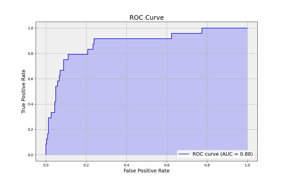
18. Area Under the Receiver Operating Characteristic (ROC) Curve (AUC-ROC)

The Area Under the Receiver Operating Characteristic (ROC) Curve, often abbreviated as AUC-ROC, is a popular performance metric used to evaluate the quality of binary classification mod e ls. The ROC curve is a graphical representation of the trade-off between the true positive rate (sensitivity or recall) and the false positive rate (1 – specificity) across various classification threshold values.

The AUC-ROC quantifies the overall ability of a classifier to distinguish between the positive and negative classes. It measures the classifier’s performance across all possible threshold values, ranging from 0 to 1. A perfect classifier would have an AUC-ROC of 1, meaning it has perfect sensitivity and specificity at all thresholds. A classifier with an AUC-ROC of 0.5 performs no better than random chance.

An example of a ROC curve, along with the corresponding AUC.

AUC-ROC has several desirable properties as a performance metric:

It is insensitive to imbalanced class distributions, as it takes into account both sensitivity and specificity.
It provides a single scalar value that summarizes the classifier’s performance across all threshold values.
It allows for easy comparison between different classifiers or classifier configurations.

However, it is important to note that AUC-ROC may not be the best metric in all situations, particularly when the costs of false positives and false negatives are very different or when there is a high class imbalance. In such cases, other metrics like precision-recall curves and F1 score might be more suitable.

19. Confusion Matrix

A Confusion Matrix is a matrix representation of a classification model’s predictions, showing the number of true positives, false positives, true negatives, and false negatives. It provides a comprehensive view of the model’s performance, allowing for the calculation of various performance metrics, such as accuracy, precision, recall, and F1 Score. By analyzing the Confusion Matrix, one can identify the model’s strengths and weaknesses and make informed decisions about potential improvements.

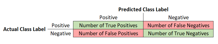
Binary confusion matrix — A representation of a confusion matrix for a binary classification problem.

20. True Positives (TP), 21. False Positives (FP), 22. True Negatives (TN), 23. False Negatives (FN)

In the context of binary classification, true positives, false positives, true negatives, and false negatives are terms used to describe the outcomes of a model’s predictions compared to the actual labels:

True Positives (TP): The number of instances where the model correctly predicts the positive class.
False Positives (FP): The number of instances where the model incorrectly predicts the positive class, while the actual label is negative.
True Negatives (TN): The number of instances where the model correctly predicts the negative class.
False Negatives (FN): The number of instances where the model incorrectly predicts the negative class, while the actual label is positive.

These outcomes form the basis for various performance metrics, such as accuracy, precision, recall, and F1 Score, used to evaluate the performance of classification models.

Some commonly used performance evaluation metrics for regression problems include:

24. Mean Absolute Error (MAE)

MAE is a regression performance metric that measures the average of the absolute differences between the predicted and actual labels. It represents the average magnitude of the errors in the model’s predictions, irrespective of their direction. The formula for MAE is:

MAE = (1/n) * Σ|y_i – ŷ_i|

where n is the number of instances, y_i is the correct label, ŷ_i is the predicted label for the ith instance, and Σ signifies summation over the n instances.

25. Mean Squared Error (MSE)

MSE is another regression performance metric that measures the average of the squared differences between the predicted and actual labels. It puts more weight on larger errors, making it more sensitive to outliers. The formula for MSE is:

MSE = (1/n) * Σ(y_i – ŷ_i)^2

where n is the number of instances, y_i is the correct label, ŷ_i is the predicted label for the ith instance, and Σ signifies summation over the n instances.

26. Root Mean Squared Error (RMSE)

RMSE is the square root of the MSE, providing an error metric in the same unit as the target variable. It combines the advantages of MSE (sensitivity to large errors) and MAE (interpretability in the same unit as the target variable). The formula for RMSE is:

RMSE = √((1/n) * Σ(y_i – ŷ_i)^2)

where n is the number of instances, y_i is the actual labe l, ŷ_i is the predicted label for the ith instance, and Σ signifies summation over the n instances.

27. R-squared (Coefficient of Determination)

R-squared is a regression performance metric that measures the proportion of the variance in the target variable that is predictable from the input features. It indicates the model’s goodness of fit and ranges from 0 to 1, with higher values indicating better performance. The formula for R-squared is:

R² = 1 – (Σ(y_i – ŷ_i)^2) / (Σ(y_i – ŷ_mean)^2)

where n is the number of instances, y_i is the correct label, ŷ_i is the predicted label for the ith instance, ŷ_mean is the mean of the correct labels, and Σ signifies summation over the n instances.

These metrics help evaluate various aspects of the model’s performance, such as its accuracy, ability to generalize, and tendency to overfit or underfit. The choice of the appropriate metric depends on the specific problem, the desired outcome, and the relative importance of different aspects of the model’s performance.

28. Learning Curve

A learning curve is a graphical representation of a model’s performance on both training and validation datasets as a function of the number of training samples or training iterations. Learning curves are useful tools for understanding the behavior of a machine learning model during the training process and diagnosing potential issues such as overfitting or underfitting.

A typical learning curve plots the training and validation performance metrics (e.g., accuracy, error, or loss) on the y-axis and the number of training samples or training iterations on the x-axis. As the model is trained with more data or for more iterations, the performance on the training set and the validation set is expected to change, revealing insights about the model’s capacity to learn and generalize.

An example of a training curve, with the training and test accuracy as a function of training epoch.

There are several key aspects to consider when analyzing a learning curve:

Convergence: Ideally, both the training and validation curves should converge to a similar performance level, indicating that the model is learning to generalize well to new data.
Gap between curves: A large gap between the training and validation curves suggests overfitting, where the model performs well on the training data but poorly on the validation data. A small gap between the curves indicates a good balance between fitting the training data and generalizing to new data.
Plateau: If both the training and validation curves plateau, it may indicate that the model has reached its capacity to learn from the data, and further training is unlikely to improve its performance.
Underfitting: If both the training and validation curves show poor performance, it suggests underfitting, meaning the model is not able to capture the underlying patterns in the data.

By analyzing the learning curve, one can gain insights into the model’s behavior and make informed decisions about the training process, such as the need for more training data, adjusting hyperparameters, changing the model architecture, or addressing issues like overfitting or underfitting.

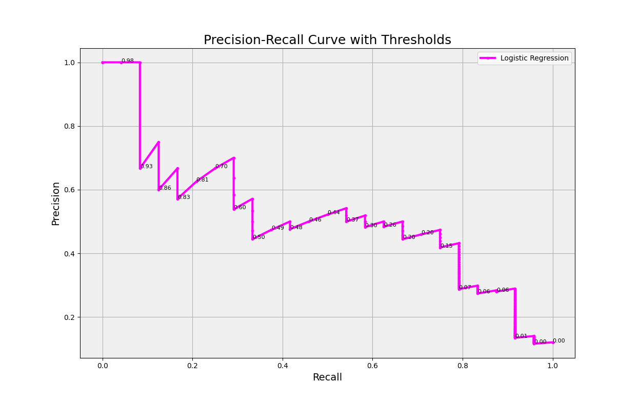
29. Precision-Recall Curve

The Precision-Recall Curve is a graphical representation of the trade-off between precision and recall for a classification model at different classification thresholds. It is a valuable tool for assessing the performance of a model, especially in situations where the dataset is imbalanced, as it focuses on the performance of the model for the positive class.

In a Precision-Recall Curve, precision is plotted on the y-axis, and recall is plotted on the x-axis. Each point on the curve corresponds to a specific classification threshold, which is the probability cutoff used by the model to classify instances as positive or negative. By adjusting the threshold, the model’s sensitivity (recall) and positive predictive value (precision) can be tuned to prioritize either one or find an optimal balance between them.

A model with perfect classification would have a curve that reaches the top right corner of the plot (precision = 1, recall = 1), while a random classifier would have a curve that follows the horizontal line at the level of the ratio of positive instances in the dataset.

An example of a precision-recall curve, with annotations for some classification threshold values.

The Precision-Recall Curve is particularly useful when comparing different models or selecting the optimal classification threshold for a specific task, considering the relative importance of precision and recall in the given context. For example, in a fraud detection scenario, a high recall might be prioritized to catch as many fraudulent cases as possible, even at the cost of some false positives, while in a medical diagnosis scenario, high precision might be prioritized to minimize false positives, which could lead to unnecessary treatments or anxiety.

30. Classification Threshold

A classification threshold, also known as a decision threshold or probability threshold, is a predefined value used in binary classification models to determine the class label of an instance based on its predicted probability. Classification models, such as logistic regression or support vector machines, typically output a probability score between 0 and 1 for each instance, indicating the likelihood that the instance belongs to the positive class.

The classification threshold is a value between 0 and 1 that acts as a cutoff for converting these probability scores into discrete class labels (positive or negative). If the predicted probability of an instance is greater than or equal to the classification threshold, the model assigns it to the positive class; otherwise, it assigns it to the negative class.

By default, a classification threshold of 0.5 is often used, meaning that instances with a predicted probability of 0.5 or higher are classified as positive, and instances with a predicted probability below 0.5 are classified as negative. However, this default threshold may not always be optimal, depending on the specific problem and the relative importance of false positives and false negatives.

Adjusting the classification threshold can help balance the trade-offs between precision, recall, and other performance metrics. A higher threshold will result in fewer false positives but more false negatives, increasing precision but reducing recall. Conversely, a lower threshold will result in more false positives but fewer false negatives, increasing recall but reducing precision.

Selecting an appropriate classification threshold depends on the specific problem and the relative costs associated with false positives and false negatives. Techniques such as the Precision-Recall curve and ROC curve can help in determining an optimal threshold based on the desired balance between these performance metrics.

31. Model selection

Model selection is the process of choosing the best machine learning model among a set of candidate models for a given problem based on their performance on unseen data. The goal of model selection is to find a model that generalizes well to new data and provides accurate predictions. Model selection is an essential step in the machine learning pipeline, as different models may perform differently depending on the characteristics of the data and the problem at hand.

The model selection process typically involves the following steps:

Define a set of candidate models: This can include different types of models (e.g., linear regression, decision trees, neural networks) or variations of the same model with different configurations (e.g., different architectures, hyperparameters).
Train and evaluate each candidate model: Each model is trained on a training dataset and evaluated on a validation dataset. Performance metrics such as accuracy, precision, recall, or F1 score for classification problems, and mean squared error, mean absolute error, or R-squared for regression problems, are used to assess the model’s performance.
Compare model performances: The performance metrics of each candidate model are compared to determine which model performs best on the validation dataset.
Select the best model: The model with the best performance on the validation dataset is chosen as the final model. In some cases, model selection may also consider factors such as model complexity, training time, and interpretability.
Validate the selected model: Once the best model is selected, it is further validated on a test dataset to obtain an unbiased estimate of its performance on unseen data.

Model selection techniques such as cross-validation, grid search, and randomized search can help automate and streamline the process of training, evaluating, and comparing candidate models. The ultimate goal of model selection is to choose a model that strikes the right balance between fitting the training data and generalizing to new, unseen data, thus avoiding issues such as overfitting or underfitting.