Gradient descent for optimization in machine learning

What is gradient descent? The short answer is, that it is an iterative algorithm for finding a local minimum of any function that is ‘smooth enough’ (a bit more precise definition for the smoothness is that the function is continuously differentiable). Another way to answer the same question briefly is by saying that gradient descent is an optimization algorithm.

Oh, and by the way, if you are wondering, finding the minimum of a function is basically the same thing as finding the maximum of a function. If you want to find the maximum of some function, but only know how to find the minimum of a function, you can simply multiply the function by -1 and then find the minimum of the new function. The maximum of the original function will be at the same coordinates as the minimum of the new function, and the maximum value of the original function will be the minimum value of the new function multiplied by -1.

If you wish to learn how gradient descent works and how to use it, you are in the right place. In this article, I will give an intuitive explanation of gradient descent that should make it easy to understand and remember. I will attempt to answer the ‘why’ in addition to the ‘how’. With this approach, I aim to teach you how you might develop the gradient descent algorithm by yourself! Furthermore, I will provide implementations for gradient descent written in Python. This should make it easy for you to get your hands dirty with gradient descent, which is in my opinion the best way to learn!

How might you find a minimum of a function?

If you are familiar with algebra, you might know that one way to find the minimum or maximum (extrema) of an objective function (the function we wish to minimize or maximize) is to find its derivative function, and then find the zeros of the derivative. The extrema of the objective function should be located in the zeros of the derivative function. However, in the real world, it is often the case that we can’t find the analytical form for the derivative function (it might be impossible or just infeasible). In these cases, we must rely on numerical approaches for finding the extrema.

Instead of finding the derivative function and its zeros, we are going to be doing something that might actually feel more intuitive. In gradient descent, we start at a random point and then follow the slope of the objective function downwards.

Think of the objective function as a landscape filled with valleys and hills. Ignoring physical constraints such as friction, if we place a ball in this landscape, we should expect that ball to roll downwards, eventually reaching the bottom of a valley, that is at least locally the lowest place in the landscape. But how can we determine what is downward for our objective function? We can use the concept of the derivative:

Derivative

The concept of the derivative comes from calculus and it’s a fundamental idea that helps us understand change. The derivative of a function provides us with the rate at which the function’s output changes with respect to its input. To put it simply, the derivative measures how sensitive a function is to changes in its input value.

Think about driving a car for example. The speedometer shows your speed, which is the rate of change of distance with respect to time. If you’re driving at a constant speed of 60 miles per hour, it means that with every ‘tiny’ change in time (every hour), your distance changes by 60 miles. In this context, 60 miles per hour is the derivative of your distance with respect to time.

Furthermore, for our purposes, the sign of the rate of change (derivative) tells us exactly what we wish to know. It tells us what is downward for our objective function. If the derivative of our objective function f(x) is positive at some point, it means that f(x) is increasing (at that point) as x increases, and so downwards is in the opposite, negative x direction, and vice versa.

Mathematically, the derivative of a function at a certain point is defined as the limit of the function’s average rate of change over an infinitesimally small interval around that point. If f(x) is our function, the derivative of f at a point x is calculated as:

f'(x) = lim(h->0) [f(x+h) - f(x)] / h

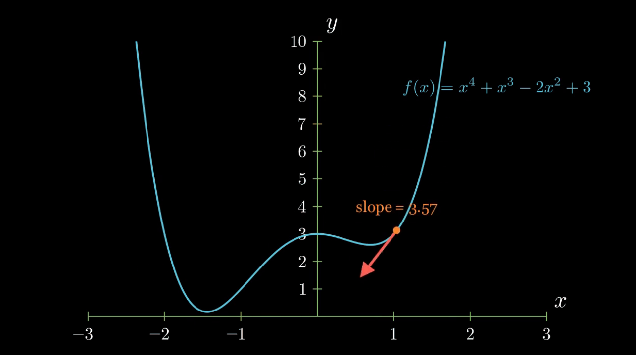
This calculation is essentially finding the slope of the line tangent to the function at the point x. This tangent line is the best linear approximation of the function near that point.

Gradient

In many real-world applications, we often encounter functions that have multiple variables. For these kinds of functions, we need a concept that is a generalization of the derivative (which is defined for single-variable functions), and this is where the gradient comes into play. The gradient of a function is a vector that stores the partial derivatives with respect to each input.

A partial derivative is a derivative taken with respect to one of the variables in a multivariable function while keeping all other variables constant. In other words, it measures how a function changes with respect to a change in one of its inputs while all other inputs remain fixed. For example, consider a function f(x, y, z), the partial derivative of f with respect to x would show how f changes when x is varied, and y and z are held constant. Similarly, the partial derivative with respect to y would show how f changes when y is varied, and x and z are held constant. These partial derivatives form the components of the gradient vector of the function, providing key information about the function’s rate and direction of change at a given point in its input space.

As the gradient is a vector, it has a direction in addition to a magnitude. The gradient vector points in the direction of the greatest rate of increase of the function, and its magnitude is the rate of increase in that direction. Conversely, moving in the opposite direction of the gradient (i.e., following the negative gradient) results in the fastest decrease of the function. This is the concept that underpins gradient descent.

So, in a way, you can think of the gradient as an extension of the derivative. If the derivative tells you how much a function changes when you nudge the input a tiny bit, the gradient tells you not only how much the function changes when you nudge the inputs, but also the direction in which you should nudge each input to get the biggest increase or decrease.

For our purposes specifically, the gradient is even better than the derivative. We wished to know what is downward for our objective function, and the negative gradient gives exactly that as the direction of the negative gradient vector. Additionally, we get the steepness of the objective function (as the magnitude of the vector), which we can use to determine how fast the ball should roll down the hill in our hills and valleys analogy.

Gradient Descent

Gradient Descent is a popular optimization algorithm used to find optimal parameters that minimize a given function. It is heavily utilized in the fields of machine learning and deep learning. Gradient descent is based on the intuition I mentioned earlier: following the negative gradient leads to the fastest decrease in the function.

Here’s how it works: we start with an initial guess for the function’s minimum. We compute the gradient at this point. Then we take a step in the direction opposite to the gradient (i.e., the direction of the steepest descent). We then compute the gradient at this new point and take another step in the direction of the steepest descent. This process is (typically) repeated until we reach a point where the gradient is approximately zero, which should be a local minimum of the function. Another stopping criterion is reaching some predetermined maximum number of iterations.

The size of each step is determined by a parameter called the learning rate. Note, that the choice of the learning rate parameter must be made carefully. If the learning rate is too high, we might step over the minimum and end up oscillating around it, or even overshoot by a huge margin and diverge further away from the minimum at each iteration. If it’s too low, the algorithm will take a long time to converge. See the animation below for a visualization of what I mean.

Overall, the gradient descent algorithm is a practical and efficient way to find good (though not always perfect) solutions to complex problems in machine learning. It’s worth noting that gradient descent only guarantees convergence to a local minimum, not necessarily the global minimum, although for many practical problems, this is often sufficient.

The formula for a single iteration of gradient descent is:

x_new = x_old - learning_rate * f'(x_old)

In this formula:

• x_old is the current point, i.e., our current estimate for the minimum of the function.
• f'(x_old) is the gradient of the objective function f evaluated at x_old. This gradient points in the direction of the steepest ascent, i.e., the direction in which the function increases the most.
• learning_rate is a positive scalar, which determines the size of the step that we take in the direction of the steepest descent (which is the opposite of the direction of steepest ascent). The learning rate is also known as the step size.
• x_new is the updated point after taking a step in the direction of the steepest descent.

This same process can be done for any function with an arbitrary number of variables (dimensions), which makes it great for optimization in high-dimensional spaces, like the hypothesis space of a neural network. In the context of optimization problems with multiple variables (like most machine learning models), x_old and x_new are vectors in a high-dimensional space, and the function f and its gradient f' are also vector-valued. The gradient descent formula is applied element-wise to each component of these vectors.

This process is repeated for a predetermined number of iterations, or until x_new and x_old are sufficiently close according to some criterion, which indicates that the algorithm has converged to a (local) minimum.

Dense fog analog:

Along with the ball rolling down the hill analog, there is another intuitive way to think about gradient descent. Consider yourself to be hiking on a range of hills when suddenly a dense fog falls upon you, and you can only see a few meters in each direction. You are at a high altitude and want to reach the bottom, where you live. What you can do is look around in your local neighborhood (which is the few meters you can see around you), and determine where the landscape is going down the fastest. If you keep moving in that direction, you will eventually reach the bottom of the range of hills (at least locally). Now you just need tp hope that you don’t get trapped in the wrong valley!

A brief detour: The Central Difference method

The central difference method is a technique used in numerical calculus to approximate the derivative/gradient of a function. The method is based on the idea that the derivative of a function at a given point is essentially the slope of the function at that point, and the slope can be approximated by looking at the function values in a small neighborhood around that point.

Here’s the general idea:

1. The derivative of a function f(x) at a point x is defined as the limit as h approaches 0 of (f(x + h) - f(x)) / h. This is the definition of a derivative, and it’s essentially the slope of a line tangent to the function at the point x.
2. But in practice, we can’t take the limit as h goes to 0 in a computer program. So instead, we choose a very small h, and calculate (f(x + h) - f(x)) / h. This is called the “forward difference” method.
3. The forward difference method is a good approximation, but it’s not symmetric about the point where we’re calculating the derivative. It only uses information about the function’s behavior after that point.
4. The “central difference” method, on the other hand, averages the forward difference and the “backward difference” ((f(x) - f(x - h)) / h) to get a more accurate and symmetric approximation: (f(x + h) - f(x - h)) / (2 * h).

So, the central difference method gives us a way to approximate the derivative of a function using the function’s values at two points: a little bit ahead of x and a little bit behind x. It tends to be more accurate than either the forward or backward difference methods, especially for small values of h. I encourage you to take another look at the first animation in this article. At the end of the animation, you can see h approaching 0 as the line becomes the tangent line of the function. The Central Difference method is simply a way of computing the slope of that tangent line.

It’s important to note that, while the central difference method can give good approximations of derivatives, it does introduce some errors, and the accuracy of the approximation can depend heavily on the choice of h. If h is too large, the approximation may be off because the function can change significantly over the interval h. If h is too small, the approximation can be thrown off by numerical precision issues because the difference between f(x + h) and f(x - h) can become very small.

Implementing gradient descent in Python

But how do you actually implement gradient descent? In this section, I will first go through an implementation of gradient descent in Python for a single variable function, where both the objective function and the gradient function are known. This is the simplest case and should serve as a good starting point for understanding the implementation of the gradient descent algorithm.

But what about functions with more than one variable?

Or what if the gradient function of the objective function is not known? After all, if the gradient function is known, couldn’t we just find the zeros of that function in order to find the extrema of the objective function? This is true. However, in real-world scenarios we rarely have the luxury of knowing the analytical form for the gradient function, and numerical methods for approximating the gradient are needed.

For these reasons, I will also provide an implementation for performing gradient descent for a two-variable function, while also approximating the gradient with something known as the central difference method (which is the simplest numerical approximation for the gradient of a function). Finally, I will provide an implementation for performing gradient descent for a function with an arbitrary number of variables, and a numerical approximation for the gradient.

Implementation for a single-variable function

Here we define a Python function grad_descent to perform the gradient descent. The parameters it takes are the function to minimize (func), the gradient of that function (grad_func), the initial point for the gradient descent (initial_point), the learning rate which determines how big a step we take downhill during each iteration (learning_rate), and the total number of iterations to run the gradient descent (num_iterations).

We then define f(x), which is the function we want to minimize, as well as df(x), its derivative. In this example f(x) is a simple quadratic equation, and df(x) is calculated analytically.

The gradient descent is initialized with a starting point and then it begins to take steps in the direction that reduces the function’s value the most. It does this for a specified number of iterations. The size of each step is determined by the learning rate and the gradient at the current point.

# Import necessary libraries
import numpy as np

def grad_descent(func, grad_func, initial_point, learning_rate=0.01, num_iterations=1000):
    """
    Gradient Descent implementation for a single-variable function.

    Parameters:
    func: The function to minimize
    grad_func: The gradient (derivative) of the function
    initial_point: The starting point for the gradient descent
    learning_rate: The learning rate (step size)
    num_iterations: The number of iterations to run the gradient descent

    Return:
    The point that (hopefully) represents the function's minimum
    """
    x = initial_point

    # Loop for the specified number of iterations
    for i in range(num_iterations):

        if i % 100 == 0:
            print("Iteration: {}\nValue of x: {:.2f}\nValue of objective function: {:.2f}".format(i,x,func(x)))

        gradient = grad_func(x)  # Calculate the gradient at the current point
        x -= learning_rate * gradient  # Take a step in the direction of steepest descent

    return x

# Define a single-variable function and its derivative
def f(x):
    return x**2 - 4*x + 4

def df(x):
    return 2*x - 4

# Use gradient descent to find the minimum
initial_point = 10.0
minimum = grad_descent(f, df, initial_point, learning_rate=0.01, num_iterations=400)

print("Minimum at x = {}\nValue of objective function: {}".format(minimum,f(minimum)))

When you run this code, you should get the following output:

Iteration: 0
Value of x: 10.00
Value of objective function: 64.00
Iteration: 100
Value of x: 3.06
Value of objective function: 1.13
Iteration: 200
Value of x: 2.14
Value of objective function: 0.02
Iteration: 300
Value of x: 2.02
Value of objective function: 0.00
Minimum at x = 2.0024746869264467
Value of objective function: 6.124075383695526e-06

You can analytically check (quite easily actually), that the minimum of the objective function is indeed located at x = 2, and at that point f(x) = 0. With the 400 iterations, we got basically there, although there is a small error left compared to the exact, analytical solution. This is very typical with numerical approaches.

I encourage you to experiment a little bit at this point. How does changing the learning_rate parameter change the speed of convergence to the correct solution? You could also try different functions.

Implementation for a two-variable function, with approximated gradient

In this code, numerical_gradient is a function that computes the gradient of func at point x using the central difference method. This method uses the average of function values at x+h and x-h to approximate the derivative. h is a very small number and is used as the step size for the finite difference.

The grad_descent function applies the gradient descent algorithm by utilizing the numerical_gradient function to compute the gradients. The gradients are used to adjust the x values in the direction that minimizes the function.

Finally, we define a function f(x, y) = x^2 + y^2 which is a simple two-variable function that we aim to minimize. In this case, we don’t need to provide the gradient function, the grad_descent algorithm can handle the computation of the gradient numerically. We initialize the gradient descent with some starting point, and it iteratively moves towards the minimum of the function.

# Import necessary libraries
import numpy as np

def numerical_gradient(func, x, h=1e-5):
    """
    Approximate gradient of a two-variable function `func` at point `x` with the central difference method.

    Parameters:
    func: The function whose gradient we want to compute
    x: The point at which to compute the gradient
    h: A small number, the step size for the finite difference
    
    Return:
    The approximated gradient vector
    """
    grad = np.zeros(2)
    fxh1 = np.zeros(2)
    fxh2 = np.zeros(2)

    for i in range(2):
        tmp = x[i]
        x[i] = tmp + h
        fxh1[i] = func(*x)

        x[i] = tmp - h
        fxh2[i] = func(*x)

        grad[i] = (fxh1[i] - fxh2[i]) / (2*h)
        x[i] = tmp  # restore original value

    return grad

def grad_descent(func, initial_point, learning_rate=0.01, num_iterations=1000):
    """
    Gradient Descent implementation for a two-variable function that uses a numerical gradient.

    Parameters:
    func: The function to minimize
    initial_point: The starting point for the gradient descent
    learning_rate: The learning rate (step size)
    num_iterations: The number of iterations to run the gradient descent
    
    Return:
    The point that (hopefully) represents the function's minimum
    """
    x = initial_point

    for i in range(num_iterations):

        if i % 100 == 0:
            print("Iteration: {}".format(i))
            print("Current point: ", x)
            print("Value of objective function: ", func(*x))

        gradients = numerical_gradient(func, x)
        x -= learning_rate * gradients  # Take the gradient step

    return x

# Define a two-variable function
def f(x, y):
    return x**2 + y**2

# Use gradient descent to find the minimum
initial_point = np.array([2.0, 2.0])
minimum = grad_descent(f, initial_point, learning_rate=0.02, num_iterations=400)

print("Minimum at ", minimum)
print("Value of objective function: ", f(*minimum))

When you run this code, you should get the following output:

Iteration: 0
Current point:  [2. 2.]
Value of objective function:  8.0
Iteration: 100
Current point:  [0.03374064 0.03374064]
Value of objective function:  0.00227686140214913
Iteration: 200
Current point:  [0.00056922 0.00056922]
Value of objective function:  6.480122305767797e-07
Iteration: 300
Current point:  [9.60284475e-06 9.60284475e-06]
Value of objective function:  1.8442925449070985e-10
Minimum at  [1.62003058e-07 1.62003058e-07]
Value of objective function:  5.248998137230217e-14

The correct minimum for this objective function is at (0,0), and the minimum is 0, meaning we once again got pretty close with the 400 iterations and the learning rate of 0.02. Once again, I encourage you to experiment with the code yourself and get your hands dirty!

Implementation for a function with an arbitrary number of variables and approximated gradient

In this code, numerical_gradient computes the gradient of func at point x using a finite difference method. For each dimension in x, it computes the function’s value at x+h and x-h, where h is a very small number. The difference between these two values, divided by 2h, is an approximation of the derivative at x.

generalized_grad_descent applies the gradient descent algorithm as before, but now it doesn’t need a grad_func parameter. Instead, it calls numerical_gradient to compute the gradients. Since numerical_gradient and func work with an arbitrary number of variables, so does generalized_grad_descent.

The example function f(x, y, z) = x^2 + y^2 + z^2 is the same as before. The difference is that now the gradient is not known in advance, and it is approximated numerically by numerical_gradient.

Remember that numerical approximation of the gradient can be less accurate and more computationally intensive than an analytic gradient. However, in many practical cases, the function to be minimized can be complex and the analytic gradient might not be readily available, which makes numerical approximation a very handy tool.

# Import necessary libraries
import numpy as np

def numerical_gradient(func, x, h=1e-5):
    """
    Approximate gradient of a multivariate function `func` at point `x` with a central difference method.

    Parameters:
    func: The function whose gradient we want to compute
    x: The point at which to compute the gradient
    h: A small number, the step size for the finite difference
    
    Returns:
    The approximated gradient vector
    """
    dim = len(x)
    grad = np.zeros(dim)
    fxh1 = np.zeros(dim)
    fxh2 = np.zeros(dim)
    for i in range(dim):
        tmp = x[i]
        x[i] = tmp + h
        fxh1[i] = func(*x)

        x[i] = tmp - h
        fxh2[i] = func(*x)

        grad[i] = (fxh1[i] - fxh2[i]) / (2*h)
        x[i] = tmp  # restore original value

    return grad

def generalized_grad_descent(func, initial_point, learning_rate=0.01, num_iterations=1000):
    """
    Generalized Gradient Descent implementation for a multi-variable function.

    Parameters:
    func: The function to minimize
    initial_point: The starting point for the gradient descent
    learning_rate: The learning rate (step size)
    num_iterations: The number of iterations to run the gradient descent
    
    Return
    The point that (hopefully) represents the function's minimum
    """
    x = initial_point

    for i in range(num_iterations):

        if i % 100 == 0:
            print("Iteration: {}".format(i))
            print("Current point: ", x)
            print("Value of objective function: ", func(*x))

        gradients = numerical_gradient(func, x)
        x -= learning_rate * gradients  # Take the gradient step

    return x

# Define a multivariate function, in this case three-variable function
def f(x, y, z):
    return x**2 - 2*x + y**2 + z**2 + z*y

# Use gradient descent to find the minimum
initial_point = np.array([2.0, -5.0, 7.0])
minimum = generalized_grad_descent(f, initial_point, learning_rate=0.05, num_iterations=400)

print("Minimum at ", minimum)
print("Value of objective function: ", f(*minimum))

When you run this code, you should get the following output:

Iteration: 0
Current point:  [ 2. -5.  7.]
Value of objective function:  39.0
Iteration: 100
Current point:  [ 1.00002656 -0.03552309  0.03552326]
Value of objective function:  -0.998738103309505
Iteration: 200
Current point:  [ 1.00000000e+00 -2.10315997e-04  2.10315998e-04]
Value of objective function:  -0.9999999557671813
Iteration: 300
Current point:  [ 1.00000000e+00 -1.24518145e-06  1.24518140e-06]
Value of objective function:  -0.9999999999984496
Minimum at  [ 1.00000000e+00 -7.37243155e-09  7.37237427e-09]
Value of objective function:  -1.0

The correct minimum for this objective function is at (1,0,0), and the minimum is -1, meaning we once again got very close with the 400 iterations and the learning rate of 0.05. Now get out there and minimize some functions!

Pros and Cons of Gradient Descent

There are many pros and cons to the gradient descent algorithm. Here are some notable ones:

Pros:

1. Simplicity: One of the primary advantages of vanilla gradient descent is its straightforwardness. It’s easy to understand and implement, especially for beginners.
2. Convergence: For convex functions and under appropriate conditions (like a suitable learning rate), vanilla gradient descent guarantees convergence to the global minimum.
3. General Applicability: It can be applied to almost any differentiable function. This means that if you can compute the gradient of a function, you can use gradient descent to find its minimum.

Cons:

1. Sensitive to Learning Rate: The convergence of vanilla gradient descent is highly sensitive to the choice of learning rate. If it’s too small, the algorithm will converge slowly. If it’s too large, it can overshoot the minimum and may not converge at all.
2. Local Minima: For non-convex functions, vanilla gradient descent can get stuck in local minima and may not find the global minimum.
3. No Adaptive Learning Rate: Unlike some advanced versions (e.g., Adagrad, RMSprop, Adam), vanilla gradient descent doesn’t adapt its learning rate during the optimization process. This non-adaptivity can lead to sub-optimal convergence speeds.
4. Scalability Issues: For large datasets, computing the gradient over the entire dataset (batch gradient descent) can be computationally expensive, leading to slow updates.
5. Poor Performance in Saddle Points: Vanilla gradient descent can be very slow in regions where the gradient is close to zero, but it’s not a minimum (saddle points).
6. Feature Scaling Dependency: The algorithm is sensitive to the scaling of features. If features are on different scales, it can lead to elongated contours of the cost function, causing slow convergence. Feature scaling (e.g., normalization or standardization) is often needed to make it work efficiently.
7. Straight-line Paths: Due to its reliance on the steepest descent (perpendicular to level sets), it can take indirect paths to the minimum in case of non-spherical contours. This can also lead to slow convergence.

In practice, while vanilla gradient descent provides foundational knowledge, many of its limitations are addressed by its variants and optimizations like momentum, Nesterov accelerated gradient, adaptive learning rates, and mini-batch processing. These enhancements often lead to faster and more robust convergence in real-world scenarios.

Variations / Extensions of the vanilla gradient descent algorithm

The standard or “vanilla” gradient descent algorithm has been improved upon in many ways to address some of its limitations. Here are some common improvements:

1. Stochastic Gradient Descent (SGD): Unlike the vanilla gradient descent which computes the gradient using the entire dataset (which can be computationally expensive for large datasets), Stochastic Gradient Descent updates the parameters by computing the gradient of the cost function with respect to a single randomly chosen data point. This makes SGD faster and capable of escaping shallow local minima more effectively due to its added noise in the update process.
2. Mini-Batch Gradient Descent: This is a trade-off between vanilla gradient descent and Stochastic Gradient Descent. In Mini-Batch Gradient Descent, the gradient of the cost function is computed for a small random sample of the data points called a mini-batch, instead of just one (as in SGD) or all (as in vanilla gradient descent). This offers a balance between the computational efficiency of SGD and the stability and convergence properties of vanilla gradient descent.
3. Momentum: This is a technique to prevent oscillations and speed up learning. It works by adding a fraction of the previous update to the current one, thus, when the algorithm has been moving in the same direction, the step size increases, leading to faster convergence.
4. Adaptive Learning Rate Methods: Methods like AdaGrad, RMSProp, Adam, etc., adjust the learning rate adaptively for each parameter. In areas where the cost function’s curvature is small (elongated bowl shape), these methods increase the learning rate to speed up convergence, and in areas where the curvature is large, they reduce the learning rate to prevent overshooting the minimum.
5. Nesterov Accelerated Gradient (NAG): NAG is a variant of momentum which has a stronger theoretical convergence guarantee for convex functions and in practice also works slightly better than standard momentum.
6. Adam: Adam (Adaptive Moment Estimation) is an update to the RMSProp algorithm, which uses running averages of both the gradients and the second moments of gradients.

These improvements are generally intended to make the gradient descent algorithm faster, more robust, and able to converge with less fine-tuning of the learning rate or the initial parameters. Most machine learning libraries have implementations for at least some of these improved versions, and you should generally prefer using those when training machine learning models. Adam is typically a great choice.